Below is a set of python codes associated with Chapter 3 of Daniele Pelliccia and David M. Paganin, “Synchrotron Light: A Physics Journey from Laboratory to Cosmos” (Oxford University Press, 2025).
In order to run any of these python codes, you will need to include the following header file.
|
1 2 3 4 5 6 7 8 9 10 11 12 13 14 15 |
import sys import numpy as np import matplotlib.pyplot as plt from mpl_toolkits.mplot3d import Axes3D import matplotlib.tri as mtri from matplotlib.patches import Circle synchrotron_style = { 'font.family': 'FreeSerif', 'font.size': 30, 'axes.linewidth': 2.0, 'axes.edgecolor': 'black', 'grid.color': '#5b5b5b', 'grid.linewidth': 1.2, } |
Plotting radial and transverse fields
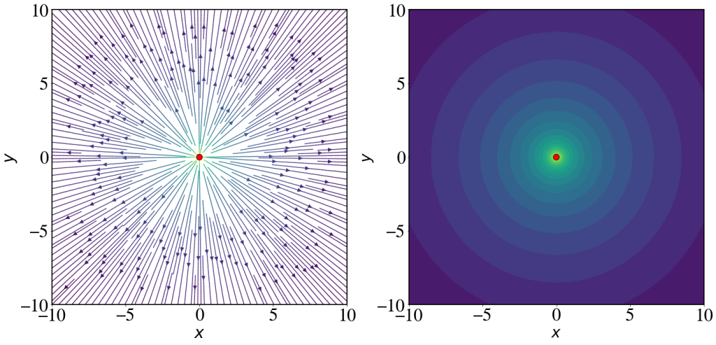
To start off, let’s work out a way to plot the electric field generated by a charge +q located at the position \mathbf{r}_{0} = (x_{0}, y_{0}). This is given by the familiar Coulomb law. The field falls off as 1/r^{2} and is directed radially outwards from the charge. We can write this in vector form:
\mathbf{E}_{r} = \frac{1}{4 \pi \epsilon_{0}} \frac{q}{\vert \mathbf{r}-\mathbf{r}_{0} \vert^{2}}\mathbf{\hat{r}}.
To draw a vector plot, we need to find an expression for the field in Cartesian coordinates. The radial unit vector can be written as a superposition of the Cartesian unit vectors as follows:
\mathbf{\hat{r}} = (\cos \Theta) \mathbf{\hat{x}} + (\sin \Theta) \mathbf{\hat{y}}.
By inverting the usual transformations in polar coordinates:
x = r\cos \Theta,y = r \sin \Theta,
we get
\cos \Theta = x/r,\sin \Theta = y/r.
Finally, by substituting in the first expression, we get the field components in Cartesian coordinates:
\mathbf{E}_{r} = \frac{1}{4 \pi \epsilon_{0}} \frac{q}{\vert \mathbf{r}-\mathbf{r}_{0} \vert^{3}}\left ( (x-x_{0})\mathbf{\hat{x}} + (y-y_{0}) \mathbf{\hat{y}} \right).
One last thing to remember is that r = \sqrt{x^{2} + y^{2}}. We can now use Numpy and Matplotlib to define and plot these functions (see Fig. 3.4).
|
1 2 3 4 5 6 7 8 9 10 11 12 13 14 |
''' Define a function that generates the electric field components as function of the charge q, position of the charge r_0 = (x_0, y_0), and the coordinate arrays x and y. To avoid potential numerical rounding errors we set 1/(4 pi epsilon_0) to be 1 ''' def E(q,r_0, x,y): den = np.hypot(x-r_0[0], y-r_0[1])**3 # denominator E_x = q * (x - r_0[0]) / den E_y = q * (y - r_0[1]) / den return E_x, E_y |
The parameters we need to pass to the streamplot function are the X and Y position, and the direction of the field E_{x} and E_{y}. The length of each arrow is proportional to the magnitude of the field at that position.
The amplitude of the field is encoded in the colour of the field lines. The large variation in magnitude of the electric field is not easily visualised using a linear scale. For this reason we define the colour scale to be the logarithm of the amplitude.
If we are only interested in a qualitative plot of the field lines, we can draw a streamplot without axes and colour bar.
|
1 2 3 4 5 6 7 8 9 10 11 12 13 14 15 16 17 18 19 20 21 22 23 24 25 26 27 28 29 30 31 32 33 34 35 36 37 38 39 40 41 42 43 44 45 46 47 48 49 50 51 52 53 54 55 56 57 58 59 60 61 62 63 64 65 66 67 68 69 70 71 72 73 |
# Plot the field generated by a charge of 1 coulomb located at the origin # Define coordinates on a grid nx, ny = 128, 128 limit = 10 x = np.linspace(-limit, limit, nx) y = np.linspace(-limit, limit, ny) X, Y = np.meshgrid(x, y) # Generate field q = 1e-9 position = [0,0] Ex, Ey = E(q, position,x=X,y=Y) # Set the colour as the amplitude of the field. We take the log to aid the visualisation. color = np.log(np.hypot(Ex, Ey)) with plt.style.context(('default')): plt.rcParams.update(synchrotron_style) # Plot the two distributions in the same figure fig, (ax1, ax2) = plt.subplots(1, 2,figsize=(20,10)) # Draw streamplot sp = ax1.streamplot(X, Y, Ex, Ey, color=color, cmap=plt.cm.viridis, \ density=3, arrowsize=1.5) # Add a circle at the position of the charge. The command "zorder" forces the circle to be on top of the lines ax1.add_artist(Circle(position, 0.02*limit, facecolor='red', edgecolor='black', zorder=10)) # Set limits and aspect ratio ax1.set_xlim(-limit,limit) ax1.set_ylim(-limit,limit) ax1.set_aspect('equal') ax1.set_xlabel('$x$', fontsize = 32) ax1.set_ylabel('$y$', fontsize = 32) ax1.set_xticks([-10,-5,0,5,10]) ax1.set_yticks([-10,-5,0,5,10]) ax1.tick_params(axis='x', labelsize = 36) ax1.tick_params(axis='y', labelsize = 36) # Add a colourbar and scale its size to match the chart size # cbar1 = fig.colorbar(sp.lines, ax = ax1, fraction = 0.046, pad = 0.04) # cbar1.ax.set_ylabel('Log Field Amplitude', fontsize = 24) # cbar1.ax.tick_params(axis='y', labelsize=18) # Draw contour plot ax2.contourf(X, Y, np.log(np.hypot(Ex, Ey)), levels=20, cmap=plt.cm.viridis) # Add a circle at the position of the charge ax2.add_artist(Circle(position, 0.02*limit, facecolor='red', edgecolor='black', zorder=10)) # Set limits and aspect ratio ax2.set_xlim(-limit,limit) ax2.set_ylim(-limit,limit) ax2.set_aspect('equal') ax2.set_xticks([-10,-5,0,5,10]) ax2.set_yticks([-10,-5,0,5,10]) ax2.set_xlabel('$x$', fontsize = 30) ax2.set_ylabel('$y$', fontsize = 30) ax2.tick_params(axis='x', labelsize=36) ax2.tick_params(axis='y', labelsize=36) # Add a colourbar and scale its size to match the chart size # cbar2 = fig.colorbar(sp.lines, ax=ax2, fraction=0.046, pad=0.04) # cbar2.ax.set_ylabel('Log Field Amplitude', fontsize = 38) # cbar2.ax.tick_params(axis='y', labelsize=30) fig.tight_layout() plt.show() |
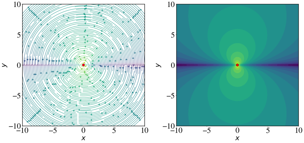
The expression we derived for the transverse field is (we suppose for simplicity that the charge is centred at the origin)
\mathbf{E}_{t} = \frac{1}{4 \pi \epsilon_{0}} \frac{qa \sin\theta}{c^{2}r}\boldsymbol{\hat{\theta}}.
Note that the direction of the transverse field, \boldsymbol{\hat{\theta}}, is by construction perpendicular to the direction of the radial field. The corresponding transformation for the angular unit vector into Cartesian coordinates is
\boldsymbol{\hat{\theta}} = (\sin \theta) \mathbf{\hat{x}} - (\cos \theta) \mathbf{\hat{y}}.
By using the transformation for polar coordinates, the transverse field in Cartesian coordinates takes the form:
\mathbf{E}_{t} = \frac{1}{4 \pi \epsilon_{0}} \frac{qa y}{c^{2}r^{3}} \left( y\mathbf{\hat{x}} - x\mathbf{\hat{y}} \right).
|
1 2 3 4 5 6 7 8 9 10 11 |
'''For simplicity and clarity, as well as avoiding potential numerical errors, we set all constants to 1. ''' def ET(q, a, x,y): den = np.hypot(x, y)**3 # denominator ET_x = -q * a * y**2 / den ET_y = q * a * y*x / den return ET_x, ET_y |
Following exactly the same steps seen before, here we draw the streamplot of the transverse field. Note, as expected, the transverse field is zero when \sin \theta = 0, i.e. in the direction of the charge acceleration. The field shows the typical ‘double-lobe’ structure.
|
1 2 3 4 5 6 7 8 9 10 11 12 13 14 15 16 17 18 19 20 21 22 23 24 25 26 27 28 29 30 31 32 33 34 35 36 37 38 39 40 41 42 43 44 45 46 47 48 49 50 51 52 53 54 55 56 57 58 59 60 61 62 63 64 65 66 67 68 |
# Define coordinates on a grid nx, ny = 128, 128 limit = 10 x = np.linspace(-limit, limit, nx) y = np.linspace(-limit, limit, ny) X, Y = np.meshgrid(x, y) # Generate field q = 1e-9 a = 1 position = [0,0] ETx, ETy = ET(q,a,x=X,y=Y) # Set the colour as the amplitude of the field. We take the log to aid the visualisation. color = np.log(np.hypot(ETx, ETy)) with plt.style.context(('default')): plt.rcParams.update(synchrotron_style) # Plot the two distributions in the same figure fig, (ax1, ax2) = plt.subplots(1, 2,figsize=(20,10)) # Draw streamplot, arrowstyle='->' sp = ax1.streamplot(X, Y, ETx, ETy, color=color, cmap=plt.cm.viridis, \ density=3, arrowsize=1.5) # Add a circle at the position of the charge. The command "zorder" forces the circle to be on top of the lines ax1.add_artist(Circle(position, 0.02*limit, facecolor='red', edgecolor='black', zorder=10)) # Set limits and aspect ratio ax1.set_xlim(-limit,limit) ax1.set_ylim(-limit,limit) ax1.set_aspect('equal') ax1.set_xlabel('$x$', fontsize = 32) ax1.set_ylabel('$y$', fontsize = 32) ax1.set_xticks([-10,-5,0,5,10]) ax1.set_yticks([-10,-5,0,5,10]) ax1.tick_params(axis='x', labelsize = 36) ax1.tick_params(axis='y', labelsize = 36) # Draw contour plot ax2.contourf(X, Y, np.log(np.hypot(ETx, ETy)), levels=20, cmap=plt.cm.viridis) # Add a circle at the position of the charge ax2.add_artist(Circle(position, 0.02*limit, facecolor='red', edgecolor='black', zorder=10)) # Set limits and aspect ratio ax2.set_xlim(-limit,limit) ax2.set_ylim(-limit,limit) ax2.set_aspect('equal') ax2.set_xticks([-10,-5,0,5,10]) ax2.set_yticks([-10,-5,0,5,10]) ax2.set_xlabel('$x$', fontsize = 32) ax2.set_ylabel('$y$', fontsize = 32) ax2.tick_params(axis='x', labelsize=36) ax2.tick_params(axis='y', labelsize=36) # Add a colourbar and scale its size to match the chart size # cbar2 = fig.colorbar(sp.lines, ax=ax2, fraction=0.046, pad=0.04) # cbar2.ax.set_ylabel('Log Field Amplitude', fontsize=38) # cbar2.ax.tick_params(axis='y', labelsize=30) fig.tight_layout() plt.show() |
Spatial distribution of emitted power in a circular accelerator
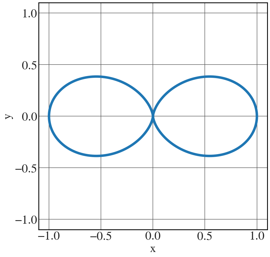
As a warm-up, we plot the 2D contours of the emitted power in the frame of reference of the moving charge, using the proportionality relation
\frac{\mathrm{d}\mathcal{P}}{\mathrm{d}\Omega} \propto \frac{q^{2} a^{2}}{c^{3}} \sin^{2} \Theta.
If we neglect the various multiplicative constants, this contour will correspond to an equation, in polar coordinates, of the type: R = \sin^{2} \Theta. This is the trick to produce this kind of contour plot in Fig. 3.6, which we’ll extend to 3D later on.
In essence, we are going to define a grid in polar coordinates and then transform to Cartesian coordinates with the constraint R = \sin^{2} \Theta.
|
1 2 3 4 5 6 7 8 9 10 11 12 13 14 15 16 17 18 19 20 21 22 23 24 25 26 27 28 |
fig = plt.figure(figsize=(9,6)) # Define an array in the space of variables theta theta = np.linspace(-np.pi, np.pi, 1000) # Set the constraint R = np.sin(theta)**2 # Define parametric equations X = R*np.sin(theta) Y = R*np.cos(theta) with plt.style.context(('seaborn-v0_8-whitegrid')): plt.rcParams.update(synchrotron_style) fig, ax = plt.subplots(figsize=(10,10)) ax.plot(X,Y, lw=6) ax.set_ylim(-1.1,1.1) ax.set_xlim(-1.1,1.1) ax.set_xlabel('x', fontsize=28) ax.set_ylabel('y', fontsize=28) ax.set_xticks([-1,-0.5,0,0.5,1]) ax.set_yticks([-1,-0.5,0,0.5,1]) plt.xticks(fontsize = 30) plt.yticks(fontsize = 30) plt.show() |
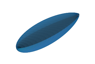
3D surface of constant power
Let’s now plot the 3D surface of constant received power (cf. Fig 3.13). The approach is exactly the same as we saw before.
Firstly we define spherical coordinates \theta and \phi. The we calculate the surface of constant power as in Eq. (3.66), which upon setting all the constants equal to one, reads:
\frac{\mathrm{d}\mathcal{P}}{\mathrm{d}\Omega} = \frac{1}{\left( 1 - \beta \cos \theta \right)^{4}} \left[ 1 - \frac{\sin^{2} \theta \cos^{2} \phi}{\gamma^{2} \left( 1 - \beta \cos \theta \right)^{2}} \right].
You can use \beta as a parameter and calculate the 3D contour as follows.
|
1 2 3 4 5 6 7 8 9 10 11 12 13 14 15 16 17 18 19 20 21 22 23 24 25 26 27 28 29 30 31 32 33 |
fig = plt.figure(figsize=(25,15)) beta = 0.9 # Change this value to produce contours for different particle speeds gamma = 1/np.sqrt(1-beta**2) # Define a mesh in the space of variables theta and phi theta = np.linspace(-np.pi, np.pi, 500) phi = np.linspace(0, np.pi, 500) T,P = np.meshgrid(theta, phi) T, P = T.flatten(), P.flatten() R = (1 - beta*np.cos(T))**(-4)*(1-np.sin(T)**2*np.cos(P)**2/(gamma**2 * (1 - beta*np.cos(T))**2)) # Define parametric equations. Note how we defined the Cartesian coordinates # in a way that is different from the usual, as a trick to produce the orientation we wish. Y = R*np.sin(T)*np.cos(P) Z = R*np.sin(T)*np.sin(P) X = R*np.cos(T) # Calculate triangles for the surface tri = mtri.Triangulation(T, P) # Plot the surface ax = fig.add_subplot(1, 1, 1, projection='3d') pl = ax.plot_trisurf(X, Y, Z, triangles=tri.triangles) ax.view_init(15, 25) ax.set_ylim(-(X.max()-X.min())/2,(X.max()-X.min())/2) #ax.set_zlim(-3000,3000) ax.set_zlim(-(X.max()-X.min())/2,(X.max()-X.min())/2) ax.set_axis_off() plt.show() |
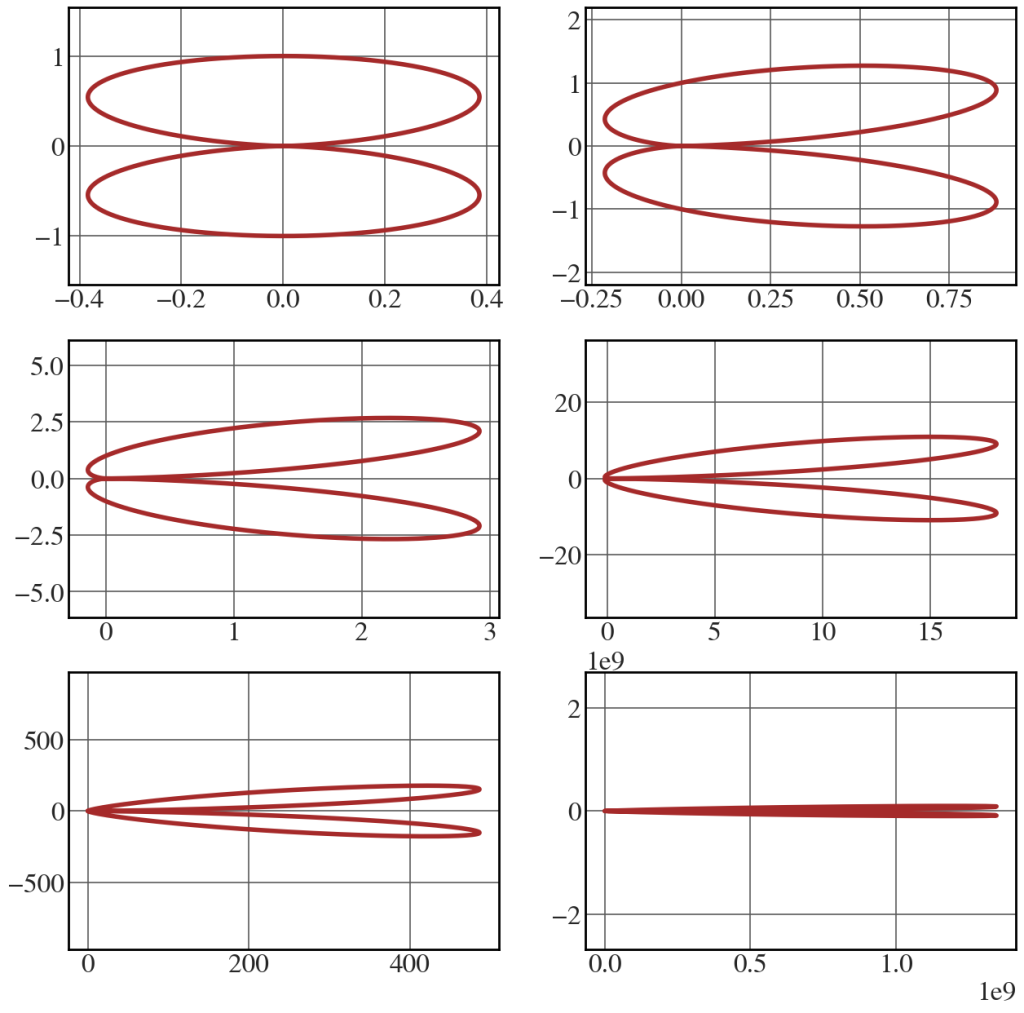
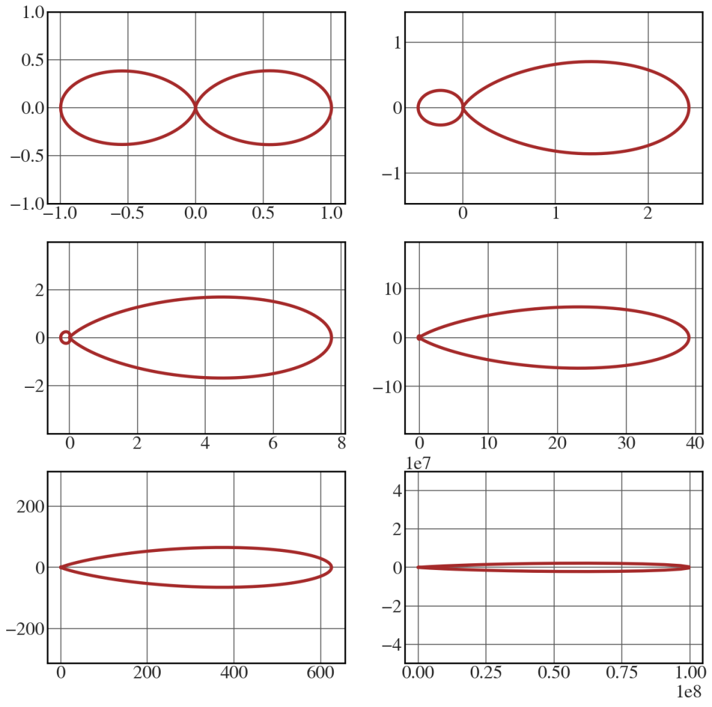
We can chart several curves at once (in 2D) by restricting ourselves to the plane \phi=0 and setting the calculation of the power distribution inside a function (see Fig. 3.15).
|
1 2 3 4 5 6 7 8 9 10 11 12 13 14 15 16 17 18 19 20 21 22 23 24 25 26 27 28 29 30 31 32 33 |
def power_distribution(beta): gamma = 1/np.sqrt(1-beta**2) # Define a mesh in the space of variables theta and phi theta = np.linspace(-np.pi, np.pi, 1000) R = (1 - beta*np.cos(theta))**(-4)*(1-np.sin(theta)**2/(gamma**2 * (1 - beta*np.cos(theta))**2)) # Define parametric equations X = R*np.cos(theta) Y = R*np.sin(theta) return (X,Y) beta = [0.001, 0.2, 0.4, 0.6, 0.8, 0.99] with plt.style.context(('seaborn-v0_8-whitegrid')): plt.rcParams.update(synchrotron_style) fig, axs = plt.subplots(nrows=3, ncols=2, figsize=(15, 15)) for i,j in enumerate(beta): ax0, ax1 = np.divmod(i,2) X,Y = power_distribution(j) axs[ax0,ax1].plot(X, Y, 'brown', lw = 4) axs[ax0,ax1].set_ylim(-(X.max()-X.min())/2,(X.max()-X.min())/2) axs[ax0,ax1].tick_params(axis='x', labelsize=24) axs[ax0,ax1].tick_params(axis='y', labelsize=24) # axs[ax0,ax1].set_title(r"$\beta=$"+str(j), y=0.85, fontsize=26) axs[ax0,ax1].xaxis.get_offset_text().set_fontsize(24) axs[ax0,ax1].yaxis.get_offset_text().set_fontsize(24) plt.show() |
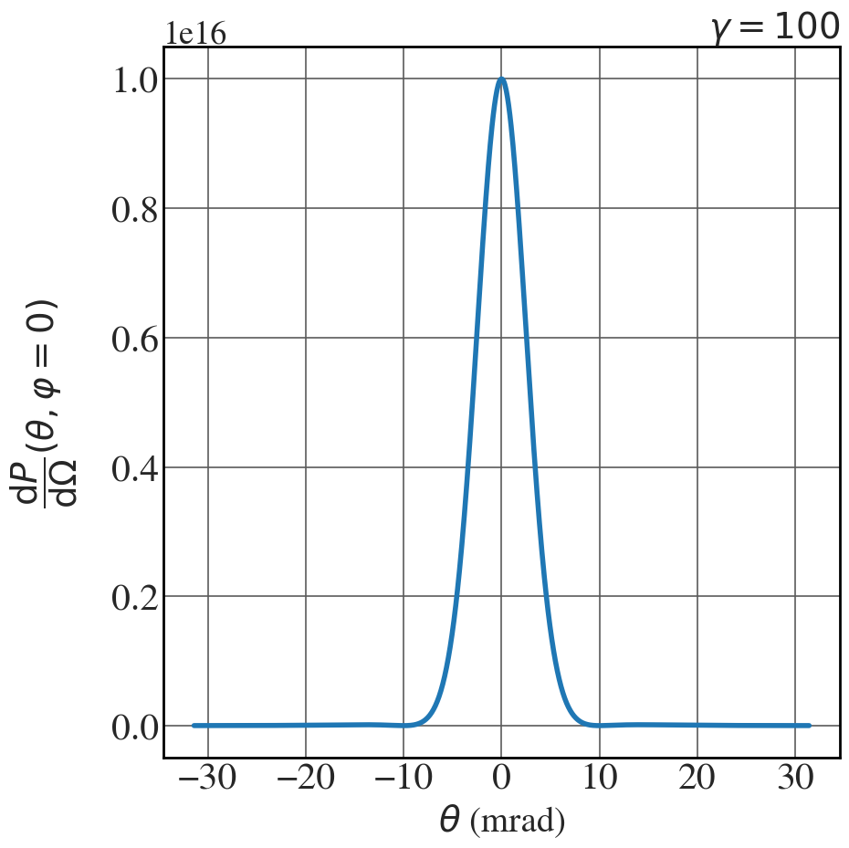
Synchrotron beam divergence in the ultra-relativistic case
The power per unit solid angle, in the limit \gamma \gg 1 , and setting all the multiplicative constants equal to one is
\frac{\mathrm{d}\mathcal{P}}{\mathrm{d}\Omega} = \frac{1}{(\theta^{2} + \gamma^{-2})^{4} } \left[ 1 - \frac{4\theta^{2}\gamma^{-2}}{(\theta^{2} + \gamma^{-2})^{2}} \right].
Here’s how to plot the graph in Fig. 3.14.
|
1 2 3 4 5 6 7 8 9 10 11 12 13 14 15 16 17 18 19 20 21 22 |
gamma = 100 theta = np.linspace(-np.pi/100, np.pi/100, 1000) P = (theta**2 + 1/gamma**2)**(-4)*(1 - (4*theta**2/gamma**2)/(theta**2 + 1/gamma**2)**2 ) with plt.style.context(('seaborn-v0_8-whitegrid')): plt.rcParams.update(synchrotron_style) fig, ax = plt.subplots(figsize=(10,10)) ax.plot(1000*theta,P, lw=4) ax.set_xlabel('$\\theta$ (mrad)', fontsize=28) ax.set_ylabel('$\\dfrac{\mathrm{d}P}{\mathrm{d}\Omega}(\\theta, \\varphi=0)$', rotation=90, fontsize=28, labelpad=25) ax.yaxis.get_offset_text().set_fontsize(26) plt.xticks(fontsize = 30) plt.yticks(fontsize = 30) ax.set_title('$\\gamma = 100$', fontsize=28, loc='right') plt.tight_layout() plt.show() |
Spatial distribution of emitted power in a linear accelerator
In this case the relevant expression is eqn (3.87). As usual we set all the multiplicative constants equal to one to get
\frac{\mathrm{d}\mathcal{P}}{\mathrm{d}\Omega} = \frac{\sin^{2}\theta}{\left( 1 - \beta \cos \theta \right)^{6}}.
|
1 2 3 4 5 6 7 8 9 10 11 12 13 14 15 16 17 18 19 20 21 22 23 24 25 26 27 28 29 30 31 |
fig = plt.figure(figsize=(15,15)) beta = 0.001 # Change this to beta = 0.9 to generate Fig. 3.16(b) gamma = 1/np.sqrt(1-beta**2) # Define a mesh in the space of variables theta and phi theta = np.linspace(-np.pi, np.pi, 500) phi = np.linspace(0, np.pi, 500) T,P = np.meshgrid(theta, phi) T, P = T.flatten(), P.flatten() R = np.sin(T)**2/(1 - beta*np.cos(T))**6 # Define parametric equations. Note how we defined the Cartesian coordinates # in a way that is different from the usual, as a trick to produce the orientation we wish. Y = R*np.sin(T)*np.cos(P) Z = R*np.sin(T)*np.sin(P) X = R*np.cos(T) # Calculate triangles for the surface tri = mtri.Triangulation(T, P) # Plot the surface. The triangles in parameter space determine which x, y, z # points are connected by an edge. ax = fig.add_subplot(1, 1, 1, projection='3d') pl = ax.plot_trisurf(X, Y, Z, triangles=tri.triangles) ax.set_xlim(-1,1) ax.set_zlim(-1,1) ax.view_init(15, 45) ax.set_axis_off() plt.show() |
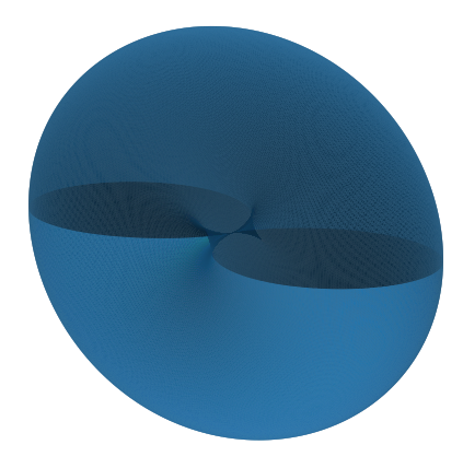
The above image coincides with Fig. 3.16(a). Below is the corresponding plot for the 2D case, as shown in Fig. 3.17.
|
1 2 3 4 5 6 7 8 9 10 11 12 13 14 15 16 17 18 19 20 21 22 23 24 25 26 27 28 29 30 31 32 |
def power_distribution_linac(beta): gamma = 1/np.sqrt(1-beta**2) # Define a mesh in the space of variables theta and phi theta = np.linspace(-np.pi, np.pi, 1000) R = np.sin(theta)**2/(1 - beta*np.cos(theta))**6 # Define parametric equations X = R*np.cos(theta) Y = R*np.sin(theta) return (X,Y) beta = [0.001, 0.2, 0.4, 0.6, 0.8, 0.99] with plt.style.context(('seaborn-v0_8-whitegrid')): plt.rcParams.update(synchrotron_style) fig, axs = plt.subplots(nrows=3, ncols=2, figsize=(15, 15)) for i,j in enumerate(beta): ax0, ax1 = np.divmod(i,2) X,Y = power_distribution_linac(j) axs[ax0,ax1].plot(X, Y, 'brown', lw = 4) axs[ax0,ax1].set_ylim(-(X.max()-X.min())/0.5,(X.max()-X.min())/0.5) axs[ax0,ax1].tick_params(axis='x', labelsize=24) axs[ax0,ax1].tick_params(axis='y', labelsize=24) axs[ax0,ax1].xaxis.get_offset_text().set_fontsize(24) axs[ax0,ax1].yaxis.get_offset_text().set_fontsize(24) plt.show() |