Below is a set of python codes associated with Chapter 10 of Daniele Pelliccia and David M. Paganin, “Synchrotron Light: A Physics Journey from Laboratory to Cosmos” (Oxford University Press, 2025).
In order to run any of these python codes, you will need to include the following header.
|
1 2 3 4 5 6 7 8 9 10 11 |
import numpy as np import matplotlib.pyplot as plt synchrotron_style = { 'font.family': 'FreeSerif', 'font.size': 30, 'axes.linewidth': 2.0, 'axes.edgecolor': 'black', 'grid.color': '#5b5b5b', 'grid.linewidth': 1.2, } |
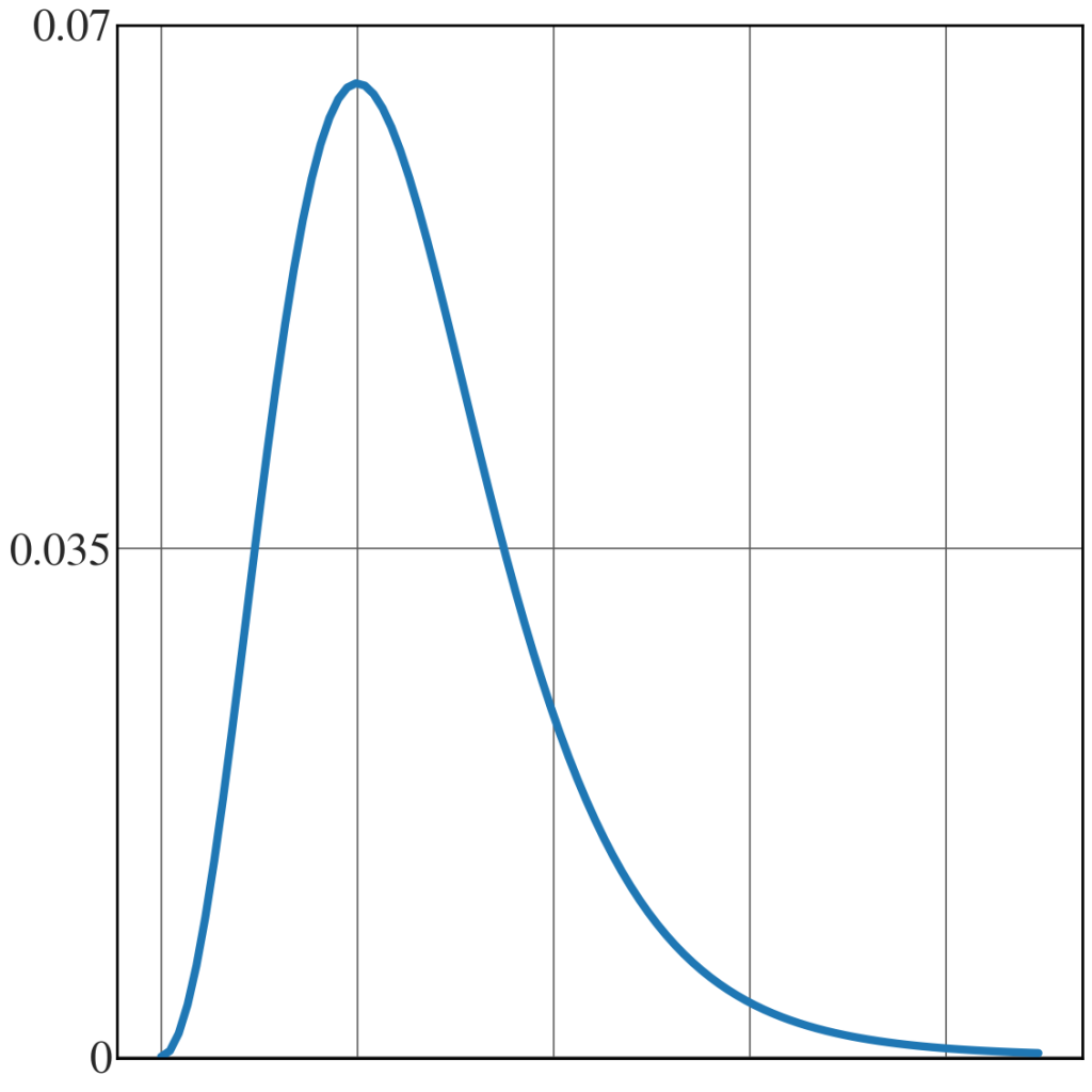
Angular dependence of classical-electrodynamics dead cone
See Fig. 10.24.
|
1 2 3 4 5 6 7 8 9 10 11 12 |
alpha = np.linspace(0,2,100) func = alpha**2 / (1 + alpha**2)**6 with plt.style.context(('seaborn-v0_8-whitegrid')): plt.rcParams.update(synchrotron_style) fig = plt.figure(figsize=(12,12)) plt.plot(alpha, func, lw = 6) plt.xticks([0, 1/np.sqrt(5), 2/np.sqrt(5), 3/np.sqrt(5), 4/np.sqrt(5)], ["", "", "", "", ""], fontsize = 26) plt.yticks([0, 0.035, 0.071], ["0", "0.035", "0.07"], fontsize = 34) plt.ylim(-0.0001,0.071) plt.tight_layout() |
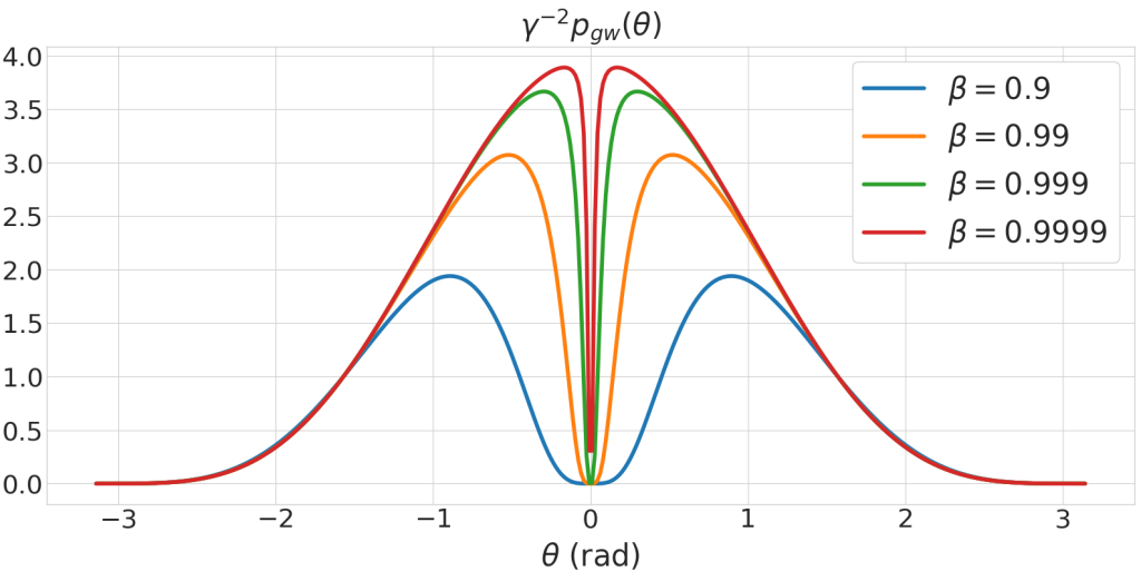
Dead cone for gravitational waves
See Fig. 10.28.
|
1 2 3 4 5 6 7 8 9 10 11 12 13 14 15 16 17 18 19 20 |
theta = np.linspace(-np.pi, np.pi, 360) beta_ = [0.9, 0.99, 0.999, 0.9999] with plt.style.context(('seaborn-v0_8-whitegrid')): # plt.rcParams.update(synchrotron_style) fig = plt.figure(figsize=(16,8.2)) for b in beta_: gamma = (1. - b**2)**(-0.5) pgw = np.sin(theta)**4 / (1.0 - b*np.cos(theta))**2 plt.plot(theta, pgw, lw = 4, label = "$\\beta=$"+str(b)) plt.legend(fontsize = 30, frameon=True, framealpha=1) plt.xticks(fontsize = 26) plt.yticks(fontsize = 26) plt.xlabel('$\\theta$ (rad)', fontsize=30, labelpad=10) plt.title("$\\gamma^{-2} p_{gw} (\\theta)$", fontsize=30) plt.tight_layout() plt.show() |