Below is a set of python codes associated with Chapter 12 of Daniele Pelliccia and David M. Paganin, “Synchrotron Light: A Physics Journey from Laboratory to Cosmos” (Oxford University Press, 2025).
In order to run any of these python codes, you will need to include the following header.
|
1 2 3 4 5 6 7 8 9 10 11 12 |
import numpy as np import matplotlib.pyplot as plt from scipy.stats import poisson synchrotron_style = { 'font.family': 'FreeSerif', 'font.size': 30, 'axes.linewidth': 2.0, 'axes.edgecolor': 'black', 'grid.color': '#5b5b5b', 'grid.linewidth': 1.2, } |
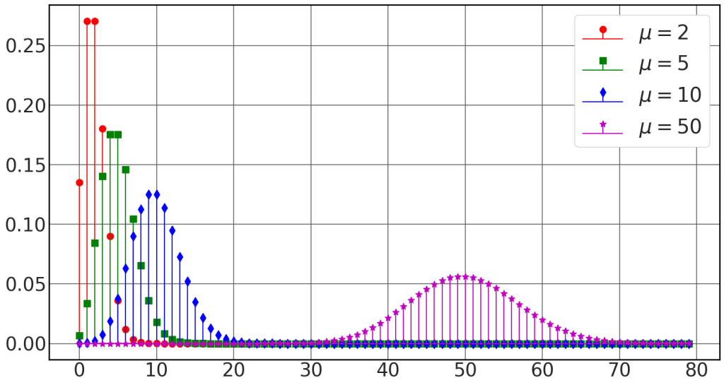
Poisson distribution
See Fig. 12.5
|
1 2 3 4 5 6 7 8 9 10 11 12 13 14 15 16 17 18 19 20 21 |
n = np.arange(0,80,1) P = np.zeros_like(n).astype('float32') linecol = ['r', 'g', 'b', 'm'] mk = ['ro','sg', 'db', '*m'] with plt.style.context(('seaborn-v0_8-whitegrid')): plt.rcParams.update(synchrotron_style) fig = plt.figure(figsize=(18,9.6)) for k, mu in enumerate([2,5,10,50]): for i,j in enumerate(n): P[i] = poisson.pmf(j, mu) markerline, stemline, baseline = plt.stem(n, P, linefmt=linecol[k], basefmt =linecol[k], markerfmt=mk[k], label="$\mu = $"+str(mu)) plt.setp(markerline, markersize = 10) plt.xticks(fontsize = 28) plt.yticks(fontsize = 28) plt.legend(fontsize=30, frameon=True, framealpha=1) plt.show() |
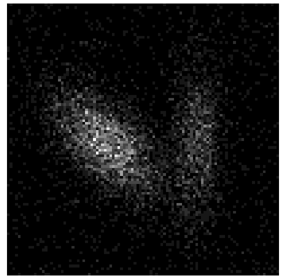
Poisson statistics
The different panels of Fig. 12.7 can be produced with the code below, by changing the value of N.
|
1 2 3 4 5 6 7 8 9 10 11 12 13 14 |
N = 5 func = 0.1+N*noiseless.reshape(-1,1).flatten() func1 = np.zeros_like(func) for i,j in enumerate(func): func1[i] = poisson.rvs(j, size=1)[0] noisy = func1.reshape(101,101) fig = plt.figure(figsize=(10,10)) plt.imshow(noisy, cmap = 'gray') plt.axis('equal') plt.axis('off') plt.show() |
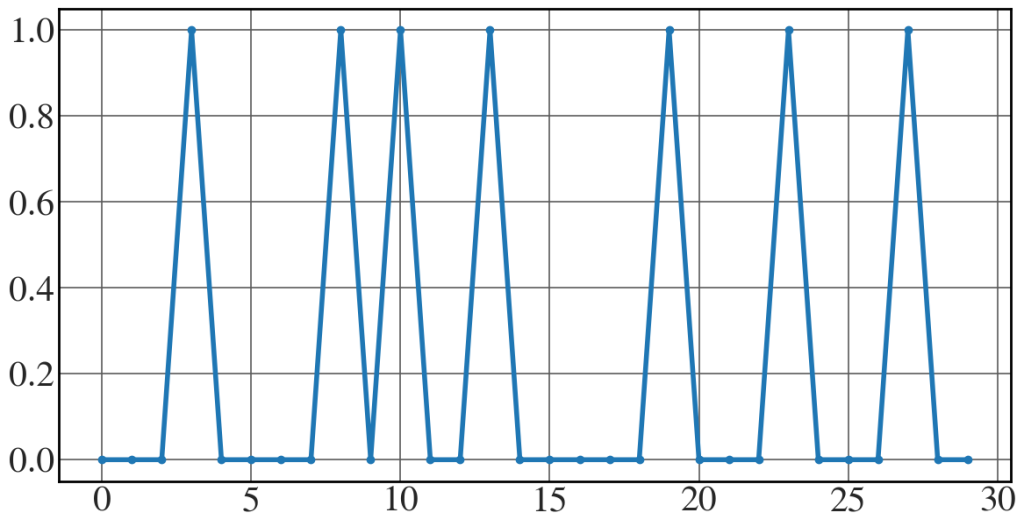
Time boxes
See Fig. 12.8.
|
1 2 3 4 5 6 7 8 |
boxes = [0,0,0,1,0,0,0,0,1,0,1,0,0,1,0,0,0,0,0,1,0,0,0,1,0,0,0,1,0,0] time = np.arange(0, len(boxes),1) with plt.style.context(('seaborn-v0_8-whitegrid')): plt.rcParams.update(synchrotron_style) fig = plt.figure(figsize=(14,7)) plt.plot(time, boxes, 'o-', lw=4) |