Below is a set of python codes associated with the Appendices of Daniele Pelliccia and David M. Paganin, “Synchrotron Light: A Physics Journey from Laboratory to Cosmos” (Oxford University Press, 2025).
In order to run any of these python codes, you will need to include the following header.
|
1 2 3 4 5 6 7 8 9 10 11 12 13 |
from scipy import special import numpy as np import matplotlib.pyplot as plt import math synchrotron_style = { 'font.family': 'FreeSerif', 'font.size': 30, 'axes.linewidth': 2.0, 'axes.edgecolor': 'black', 'grid.color': '#5b5b5b', 'grid.linewidth': 1.2, } |
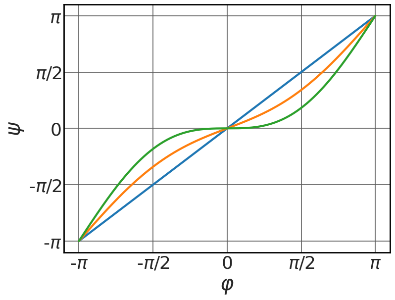
Appendix A: transformation linking the angular variables \varphi and
\psi
See Fig. A.1
|
1 2 3 4 5 6 7 8 9 10 11 12 13 14 15 |
phi = np.linspace(-np.pi, np.pi, 361) with plt.style.context(('seaborn-v0_8-whitegrid')): plt.rcParams.update(synchrotron_style) fig = plt.figure(figsize=(8.5,6.5)) for eps in [0, 0.5, 0.999]: plt.plot(phi, phi-eps*np.sin(phi), lw=3) plt.xticks([-np.pi, -np.pi/2, 0, np.pi/2, np.pi], ['-$\\pi$', '-$\\pi/2$', '0', '$\\pi/2$', '$\\pi$'], fontsize = 26) plt.yticks([-np.pi, -np.pi/2, 0, np.pi/2, np.pi], ['-$\\pi$', '-$\\pi/2$', '0', '$\\pi/2$', '$\\pi$'], fontsize = 26) plt.grid(True) plt.xlabel('$\\varphi$') plt.ylabel('$\\psi$') plt.show() |
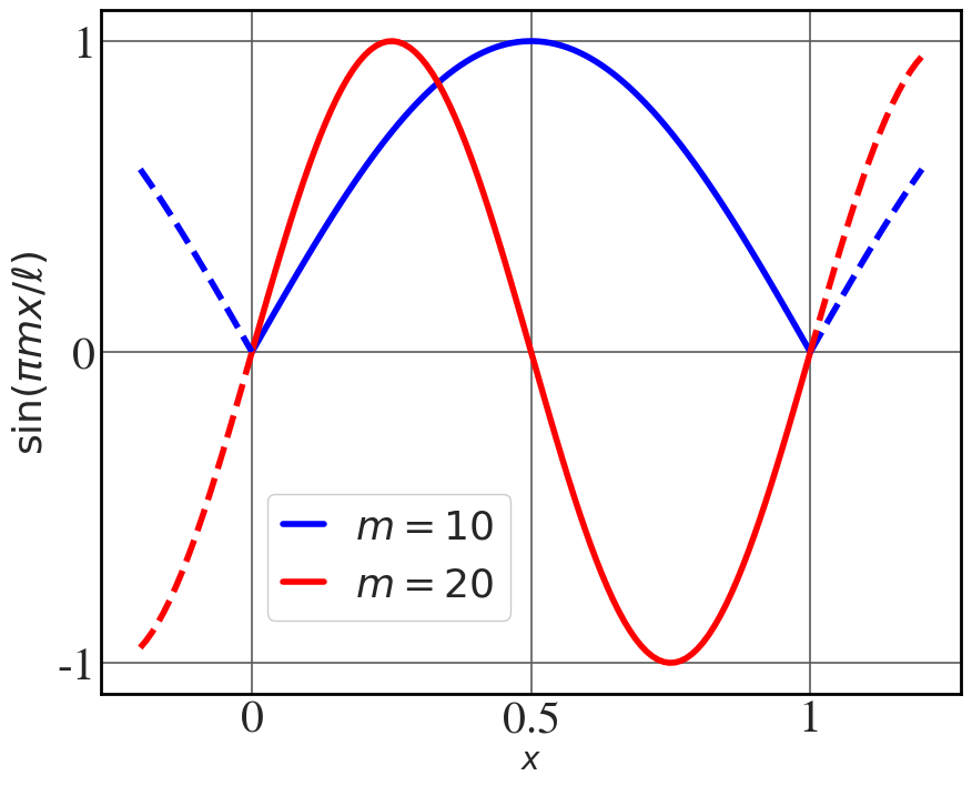
Appendix B: Boundary conditions for perfectly reflecting cavity walls
See Fig. B.1.
|
1 2 3 4 5 6 7 8 9 10 11 12 13 14 15 16 17 18 19 20 21 22 23 24 25 |
ell = 1 m = 1 x1 = np.linspace(-0.2, 0, 20) x0 = np.linspace(0, ell, 100) x2 = np.linspace(ell, 1.2, 20) with plt.style.context(('seaborn-v0_8-whitegrid')): plt.rcParams.update(synchrotron_style) fig, ax = plt.subplots(1, 1,figsize=(10,8)) plt.plot(x0, np.sin(np.pi*m*x0/1), 'b', lw=4, label = "$m=10$") plt.plot(x0, np.sin(2*np.pi*m*x0/1), 'r', lw=4, label = "$m=20$") plt.plot(x2, -np.sin(np.pi*m*x2/1), 'b--', lw=4) plt.plot(x1, -np.sin(np.pi*m*x1/1), 'b--', lw=4) plt.plot(x2, np.sin(2*np.pi*m*x2/1), 'r--', lw=4) plt.plot(x1, np.sin(2*np.pi*m*x1/1), 'r--', lw=4) ax.set_xticks([0,0.5,1]) ax.set_xticklabels(["0", "0.5", "1"], fontsize=30) ax.set_yticks([-1,0, 1]) ax.set_yticklabels(["-1", "0","1"], fontsize=30) plt.xlabel('$x$', fontsize=20) plt.ylabel('$\\sin(\\pi mx/\\ell)$', fontsize=26) plt.legend(fontsize=26, handlelength=1, frameon=True, framealpha=1, \ loc = 'center left', bbox_to_anchor=(0.17, 0.2)) plt.show() |
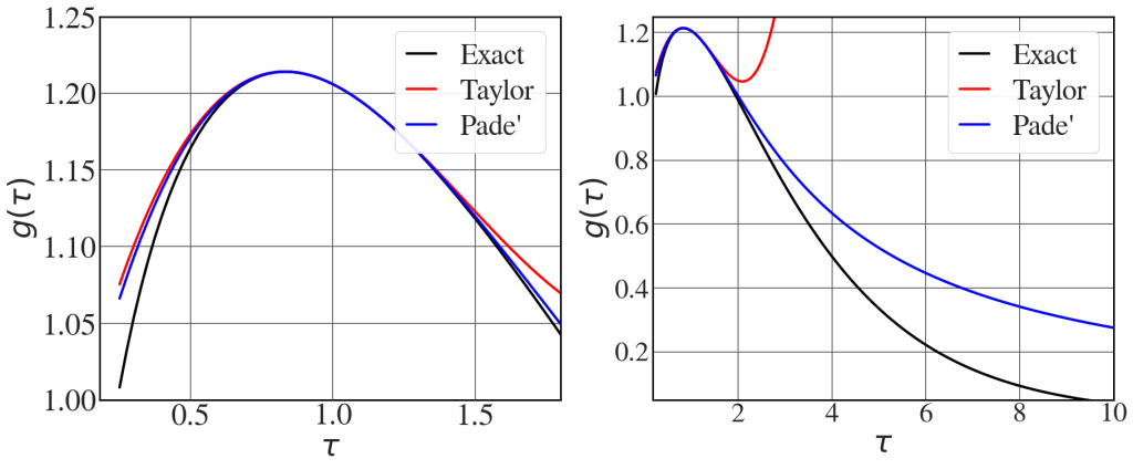
Appendix D: Relation between Taylor and Padé coefficients of g(\tau)
Calculation leading to the plot in Fig. D.1. See also Fig. 4.23.
|
1 2 3 4 5 6 7 8 9 10 11 12 13 |
def cn_recursive(n): # Base case: c_0 = 0 if n == 0: return 0 # Recursive case: c_n = c_{n-1}/2 + 1/2^(n-1) else: return 0.5*cn_recursive(n-1) + 1/2**(n-1) def derivative_K(z, N): if N == 0: return z*special.kv(2/3,z/2) else: return cn_recursive(N)*special.kvp(2/3,z/2,n=N-1) + (z/2**N)*special.kvp(2/3,z/2,n=N) |
|
1 2 3 4 5 6 7 8 9 10 11 12 13 14 15 16 17 18 19 20 21 22 23 24 25 26 27 28 29 30 31 32 33 34 35 36 37 38 39 40 41 42 43 44 45 46 47 48 49 |
x = np.linspace(0.25,10.25,401) # Point of maximum point_max = np.argmax(x*special.kv(2/3,x/2)) # Calculate the Taylor series up the the order ord ord = 4 a = np.zeros(ord) tayl_exp = np.zeros_like(x) for i in range(ord): test = derivative_K(x, i) a[i] = test[30]/math.factorial(i) tayl_exp += a[i]*(x-x[30])**i A = a[0] D = (a[2]**2 - a[3]*a[1]) / (a[1]**2 -a[2]*a[0]) C = -a[0]*D/a[1] - a[2]/a[1] B = a[1]+a[0]*C xmax = 1.0+(np.sqrt(A**2*D**2 + B*D*(B-A*C)) - A*D)/(B*D) pade = (A+B*(x-1)) / (1+C*(x-1)+D*(x-1)**2) with plt.style.context(('seaborn-v0_8-whitegrid')): plt.rcParams.update(synchrotron_style) fig, axs = plt.subplots(1,2, figsize=(21,8)) axs[0].plot(x, x*special.kv(2/3,x/2), 'k', lw=3,label = "Exact") axs[0].plot(x, tayl_exp, 'r', lw=3,label="Taylor") axs[0].plot(x, pade, 'b', lw=3,label="Pade'") axs[0].set_xlim([0.18, 1.8]) axs[0].set_ylim([1, 1.25]) axs[0].tick_params(axis='x', labelsize=36) axs[0].tick_params(axis='y', labelsize=36) axs[0].set_xlabel('$\\tau$', fontsize=36) axs[0].set_ylabel("$g(\\tau)$", fontsize=36) axs[0].legend(fontsize = 34, frameon=True, framealpha=0.9, loc = 'upper right', labelspacing=0.3, handlelength=1) axs[1].plot(x, x*special.kv(2/3,x/2), 'k', lw=3,label = "Exact") axs[1].plot(x, tayl_exp, 'r', lw=3,label="Taylor") axs[1].plot(x, pade, 'b', lw=3,label="Pade'") axs[1].set_xlim([0.18, 10]) axs[1].set_ylim([0.05, 1.25]) axs[1].tick_params(axis='x', labelsize=32) axs[1].tick_params(axis='y', labelsize=32) axs[1].set_xlabel('$\\tau$', fontsize=36) axs[1].set_ylabel("$g(\\tau)$", fontsize=36) axs[1].legend(fontsize = 34, frameon=True, framealpha=0.9, labelspacing=0.3, handlelength=1) plt.show() |