Below is a set of python codes associated with Chapter 6 of Daniele Pelliccia and David M. Paganin, “Synchrotron Light: A Physics Journey from Laboratory to Cosmos” (Oxford University Press, 2025).
In order to run any of these python codes, you will need to include the following header file.
|
1 2 3 4 5 6 7 8 9 10 11 |
import numpy as np import matplotlib.pyplot as plt synchrotron_style = { 'font.family': 'FreeSerif', 'font.size': 30, 'axes.linewidth': 2.0, 'axes.edgecolor': 'black', 'grid.color': '#5b5b5b', 'grid.linewidth': 1.2, } |
Compton scattering
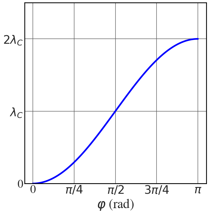
Increase in wavelength of a photon undergoing Compton scattering, as in Fig. 6.4
|
1 2 3 4 5 6 7 8 9 10 11 12 13 14 15 16 17 18 19 20 21 22 23 24 25 26 27 |
h = 6.62607015e-34 # J/Hz ee = 1.602176634e-19 C hbar = h/(2*np.pi) me = 9.11e-31 # kg c = 2.99792458e8 # m/s, speed of light lambda_c = h/(me*c) B_star = me**2 * c**2 / (ee*hbar) phi = np.linspace(0, np.pi, 100) delta_l = 2*lambda_c*np.sin(phi/2)**2 with plt.style.context(('seaborn-v0_8-whitegrid')): plt.rcParams.update(synchrotron_style) fig, axs = plt.subplots(1, 1,figsize=(8,8)) axs.plot(phi, delta_l, 'b', lw = 4) axs.tick_params(axis='x', labelsize=20) axs.tick_params(axis='y', labelsize=20) axs.set_xlabel('$\\varphi$ (rad)', fontsize=32, labelpad = 5) axs.set_xticks([0, np.pi/4, np.pi/2, 3*np.pi/4, np.pi]) axs.set_xticklabels(["0", "$\\pi/4$","$\\pi/2$","$3\\pi/4$","$\\pi$"], fontsize=28) axs.set_yticks([0, lambda_c, 2*lambda_c]) axs.set_yticklabels(["0", "$\\lambda_{C}$","$2\\lambda_{C}$"], fontsize=28) axs.set_ylim(0, 2.5*lambda_c) plt.show() |
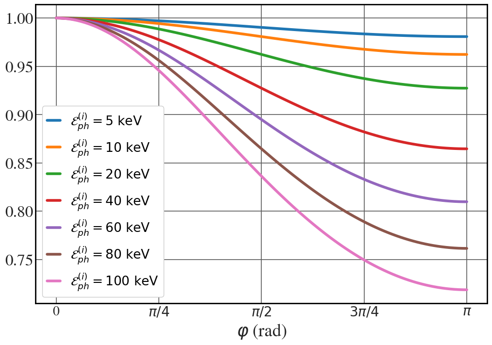
Fractional energy change for a photon undergoing Compton scattering, as in Fig. 6.5.
|
1 2 3 4 5 6 7 8 9 10 11 12 13 14 15 16 |
phi = np.linspace(0, np.pi, 100) with plt.style.context(('seaborn-v0_8-whitegrid')): plt.rcParams.update(synchrotron_style) fig, axs = plt.subplots(1, 1,figsize=(12,8)) for E_ph in [5,10,20,40,60,80,100]: axs.plot(phi, 1.0/(1+2*E_ph/511*np.sin(phi/2)**2), lw = 4, label="$\\mathcal{E}_{ph}^{(i)}=$"+str(E_ph)+" keV") axs.tick_params(axis='x', labelsize=24) axs.tick_params(axis='y', labelsize=24) axs.set_xlabel('$\\varphi$ (rad)', fontsize=26, labelpad = 5) axs.set_xticks([0, np.pi/4, np.pi/2, 3*np.pi/4, np.pi]) axs.set_xticklabels(["0", "$\\pi/4$","$\\pi/2$","$3\\pi/4$","$\\pi$"], fontsize=20) plt.legend(fontsize=19, framealpha=1, handlelength=1) plt.show() |
Inverse Compton scattering
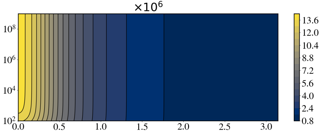
Contour plots of the relative energy boost for a photon undergoing inverse Compton scattering, as in Fig. 6.7.
|
1 2 3 4 5 6 7 8 9 10 11 12 13 14 15 16 17 18 19 20 21 22 23 24 25 26 27 28 29 30 31 32 33 34 |
gamma_e = 2 # Change this value to generate the other panels in Fig. 6.7 if gamma_e == 2: phi = np.linspace(0, np.pi, 2000) if gamma_e == 1000: phi = np.linspace(0, 0.005, 2000) if gamma_e == 10000: phi = np.linspace(0, 0.0007, 2000) lambda_ratio = np.logspace(2,9,1000) e_ratio = np.zeros((lambda_ratio.shape[0],phi.shape[0])) for i in range(lambda_ratio.shape[0]): for j in range(phi.shape[0]): e_ratio[i,j] = (np.sqrt(1-1/gamma_e**2) + 1) / \ (1- np.cos(phi[j])*np.sqrt(1-1/gamma_e**2) + (1+np.cos(phi[j]))/(gamma_e*lambda_ratio[i]) ) if gamma_e == 2: xscale = phi else: xscale = 1000*phi with plt.style.context(('default')): plt.rcParams.update(synchrotron_style) fig, axs = plt.subplots(1, 1,figsize=(18,6)) cs = axs.contourf(xscale,lambda_ratio, e_ratio, cmap='cividis',levels=20) axs.contour(xscale,lambda_ratio, e_ratio, levels=20, colors='k') axs.set_yscale('log') axs.tick_params(axis='x', labelsize=30) axs.tick_params(axis='y', labelsize=30) #axs.yaxis.get_offset_text().set_fontsize(20) plt.title("$\\times 10^{6}$") cbar = fig.colorbar(cs) cbar.ax.tick_params(labelsize=30) plt.show() |
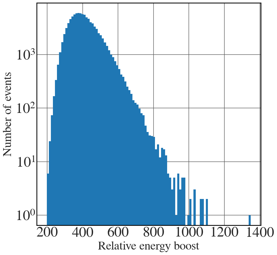
Simulating the energy distribution of an electron bunch undergoing inverse Compton scattering
Computational exercise on page 199 and Fig. 6.8.
|
1 2 3 4 5 6 7 8 9 10 11 12 13 14 15 16 17 18 19 20 21 22 23 24 25 26 27 28 29 30 |
lambdaC = 2.42631023867e-3 #nm lambda_i = 632.8 sig_laser = 0.002 gamma_e = 1000 sigma_gamma = 1 phi = 0.1 sigma_phi = 0.01 n_events = 100000 lambda_laser = lambda_i+sig_laser*np.random.normal(size=n_events) gamma_electr = gamma_e+sigma_gamma*np.random.normal(size=n_events) angle = phi + sigma_phi*np.random.normal(size=n_events) en_boost = [] for i in range(n_events): sq = np.sqrt(1-1/gamma_electr[i]**2) sf = (1 + np.cos(angle[i])) / (gamma_electr[i]*lambda_laser[i]/lambdaC) en_boost.append( ((sq + 1) / (1-sq*np.cos(angle[i]) + sf))) with plt.style.context(('seaborn-v0_8-whitegrid')): plt.rcParams.update(synchrotron_style) fig, ax = plt.subplots(figsize=(10,10)) plt.hist(en_boost, bins=100, log=True) plt.xticks(fontsize = 36) plt.yticks(fontsize = 36) plt.xlabel("Relative energy boost") plt.ylabel("Number of events") plt.show() |
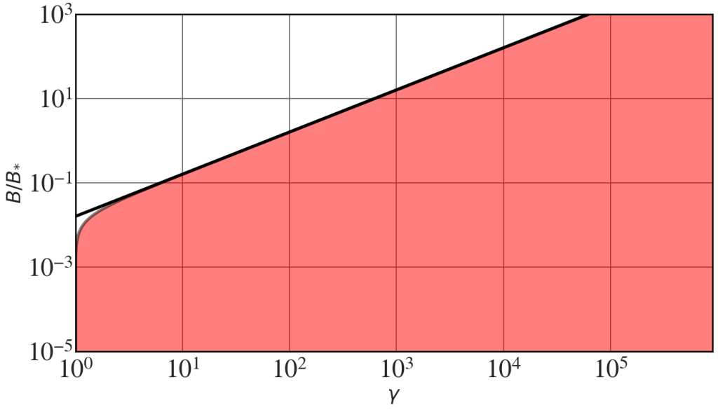
Parameter-space plots for domain of validity of classical synchrotron-light theory
Bohr synchrotron (see Fig. 6.10).
|
1 2 3 4 5 6 7 8 9 10 11 12 13 14 15 16 17 18 19 20 21 22 |
alpha = 0.007297 gamma = np.logspace(0,6, 2000) B_ratio = alpha**2 *gamma/10 with plt.style.context(('seaborn-v0_8-whitegrid')): plt.rcParams.update(synchrotron_style) fig, axs = plt.subplots(1, 1,figsize=(15,8)) #axs.loglog(gamma, B_ratio,lw = 4) axs.fill_between(gamma, B_ratio, y2=0, lw=4, edgecolor = 'k', alpha=0.5, facecolor='red') #zorder=2, axs.set_xscale('log') axs.set_yscale('log') axs.tick_params(axis='x', labelsize=34, pad=10) axs.tick_params(axis='y', labelsize=34) axs.set_xlim(1,900000) axs.set_xlabel('$\\gamma$', fontsize=26, labelpad = 5) axs.set_ylabel('$B/B_{*}$', fontsize=26, labelpad = 5) plt.show() |
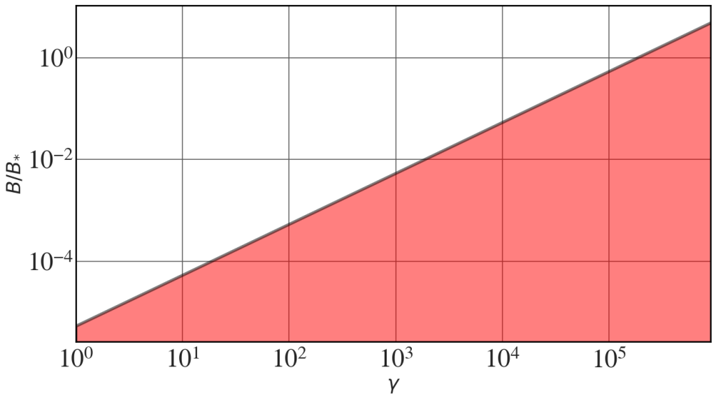
Electron recoil (see Fig. 6.11).
|
1 2 3 4 5 6 7 8 9 10 11 12 13 14 15 16 17 18 19 20 21 22 23 |
alpha = 0.007297 gamma = np.logspace(0,6, 2000) B_ratio = 0.1*np.sqrt(1. - 1.0/gamma**2)/gamma with plt.style.context(('seaborn-v0_8-whitegrid')): plt.rcParams.update(synchrotron_style) fig, axs = plt.subplots(1, 1,figsize=(15,8)) axs.plot(gamma, 0.1*(1/(gamma)), lw=4, color='k' ) axs.fill_between(gamma, B_ratio, y2=0, lw=4, edgecolor = 'k', alpha=0.5, facecolor='red') #zorder=2, axs.set_xscale('log') axs.set_yscale('log') axs.tick_params(axis='x', labelsize=34, pad=10) axs.tick_params(axis='y', labelsize=34) axs.set_xlim(1,900000) axs.set_ylim(0.0000001,1) axs.set_xlabel('$\\gamma$', fontsize=26, labelpad = 5) axs.set_ylabel('$B/B_{*}$', fontsize=26, labelpad = 5) plt.show() |
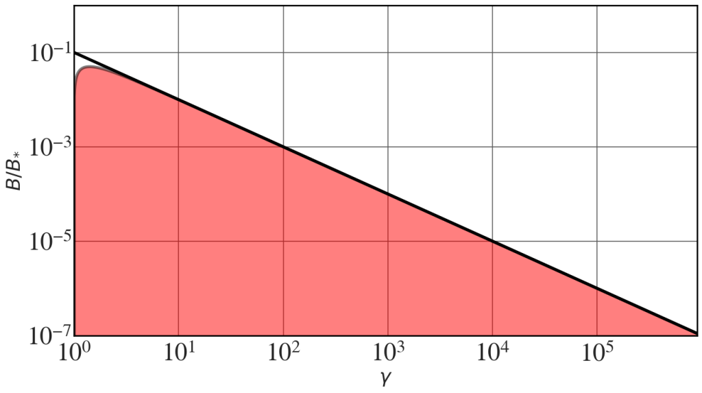
Compton wavelength (see Fig. 6.12).
|
1 2 3 4 5 6 7 8 9 10 11 12 13 14 15 16 17 18 19 20 21 22 23 |
alpha = 0.007297 gamma = np.logspace(0,6, 2000) B_ratio = 0.1*gamma*np.sqrt(1. - 1.0/gamma**2) /(2*np.pi) with plt.style.context(('seaborn-v0_8-whitegrid')): plt.rcParams.update(synchrotron_style) fig, axs = plt.subplots(1, 1,figsize=(15,8)) axs.plot(gamma, 0.1*(gamma/(2*np.pi)), lw=4, color='k' ) axs.fill_between(gamma, B_ratio, y2=0, lw=4, edgecolor = 'k', alpha=0.5, facecolor='red') #zorder=2, axs.set_xscale('log') axs.set_yscale('log') axs.tick_params(axis='x', labelsize=34, pad=10) axs.tick_params(axis='y', labelsize=34) axs.set_xlim(1,900000) axs.set_ylim(0.00001,1000) axs.set_xlabel('$\\gamma$', fontsize=26, labelpad = 5) axs.set_ylabel('$B/B_{*}$', fontsize=26, labelpad = 5) plt.show() |
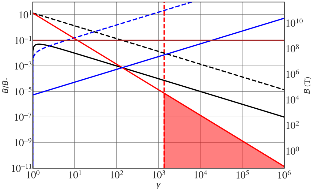
Parameter space plots of all curves which indicate the region where classical synchrotron theory is valid, as in Fig. 6.13.
|
1 2 3 4 5 6 7 8 9 10 11 12 13 14 15 16 17 18 19 20 21 22 23 24 25 26 27 28 29 30 31 32 33 34 35 36 37 38 39 40 41 42 43 44 |
def ratio2Bstar(x): return x * B_star def Bstar2ratio(x): return x / B_star alpha = 0.007297 gamma = np.logspace(0,7, 2000) mask = gamma > 10/alpha curve_I = 0.1*np.sqrt(1. - 1.0/gamma**2)/gamma curve_III = 0.1*gamma*np.sqrt(1. - 1.0/gamma**2) /(2*np.pi) curve_VI = 0.1*1.0/(alpha*gamma) curve_VII = 0.1*1.0/(alpha*gamma**2) curve_VIII = 0.1*alpha**2 *gamma curve_IX = 0.1*np.ones_like(gamma) with plt.style.context(('seaborn-v0_8-whitegrid')): plt.rcParams.update(synchrotron_style) fig, axs = plt.subplots(figsize=(15,10)) axs.plot(gamma, curve_I, lw=4, color='k' ) axs.plot(gamma, curve_III, lw=4, color='b', linestyle='dashed' ) axs.plot([10/alpha, 10/alpha], [1e-12, 100], lw=4, color='red', linestyle='dashed' ) # curve_V axs.plot(gamma, curve_VI, lw=4, color='k', linestyle='dashed' ) axs.fill_between(gamma, curve_VII, lw=4, color='red', alpha=0.5, where=mask) axs.plot(gamma, curve_VII, lw=4, color='r') axs.plot(gamma, curve_VIII, lw=4, color='b' ) axs.plot(gamma, curve_IX, lw=4, color='brown' ) axs.set_xscale('log') axs.set_yscale('log') axs.tick_params(axis='x', labelsize=34, pad=10) axs.tick_params(axis='y', labelsize=34) axs.set_xlim(1,1000000) axs.set_ylim(1e-11,100) axs.set_ylabel("$B/B_{*}$", fontsize = 26) axs.set_xlabel("$\gamma$", fontsize = 26) secax = axs.secondary_yaxis('right', functions=(ratio2Bstar, Bstar2ratio)) secax.set_ylabel("$B$ (T)", fontsize = 26) secax.tick_params(axis='y', labelsize=34) plt.show() |