Below is a set of python codes associated with Chapter 8 of Daniele Pelliccia and David M. Paganin, “Synchrotron Light: A Physics Journey from Laboratory to Cosmos” (Oxford University Press, 2025).
In order to run any of these python codes, you will need to include the following header.
|
1 2 3 4 5 6 7 8 9 10 11 12 13 14 15 |
import numpy as np import matplotlib.pyplot as plt from matplotlib.patches import Circle from matplotlib.patches import Ellipse from scipy.integrate import odeint import math synchrotron_style = { 'font.family': 'FreeSerif', 'font.size': 30, 'axes.linewidth': 2.0, 'axes.edgecolor': 'black', 'grid.color': '#5b5b5b', 'grid.linewidth': 1.2, } |
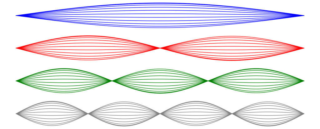
Spatial modes
See Fig. 8.1.
|
1 2 3 4 5 6 7 8 9 10 11 12 13 14 15 16 17 |
x = np.linspace(0, 2*np.pi, 1000) t1 = np.sin(x/2) t2 = np.sin(x) t3 = np.sin(3*x/2) t4 = np.sin(4*x/2) t = [t1,t2,t3,t4] colors = ['blue', 'red', 'green', 'gray'] fig, ax = plt.subplots(4, 1,figsize=(25,10), sharex=True) for i in range(1,11,1): for j in range(4): ax[j].plot(x, np.cos(np.pi*i/11)*t[j], lw = 2, color=colors[j]) for j in range(4): ax[j].plot(x, t[j], lw = 2, color=colors[j]) ax[j].set_axis_off() plt.show() |
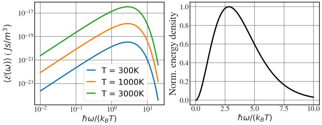
Planck’s law
See Fig. 8.2.
|
1 2 3 4 5 6 7 8 9 10 11 12 13 14 15 16 17 18 19 20 21 22 23 24 25 |
h = 6.62607015e-34 # Planck's constant hbar = h/(2*np.pi) kB = 1.380649e-23 # Boltzmann's constant c = 3.0e8 with plt.style.context(('seaborn-whitegrid')): plt.rcParams.update(synchrotron_style) fig, axs = plt.subplots(1, 2,figsize=(16.5,6)) for T in [300, 1000, 3000]: om = np.linspace(0.01*kB*T/hbar, 20*kB*T/hbar, 10000) en_density = (hbar*om**3/(np.pi**2 * c**3))/( np.exp(hbar*om/(kB*T)) -1) axs[0].loglog(hbar*om/(kB*T), en_density, lw = 4, label="T = "+str(T)+"K") axs[0].tick_params(axis='y', labelsize=24) axs[0].tick_params(axis='x', labelsize=24, pad=5) axs[0].set_ylabel('$\\langle \\mathcal{E}(\\omega)\\rangle$ ( $J s / m^{3})$', fontsize=28, labelpad = 15) axs[0].set_xlabel('$\\hbar \\omega / (k_{B}T)$', fontsize=26) axs[1].plot(hbar*om[:5000]/(kB*T), en_density[:5000]/en_density[:5000].max(), 'k', lw=4) axs[1].tick_params(axis='y', labelsize=24) axs[1].tick_params(axis='x', labelsize=24) axs[1].set_ylabel('Norm. energy density', fontsize=32) axs[1].set_xlabel('$\\hbar \\omega / (k_{B}T)$', fontsize=26) axs[0].legend(fontsize=26, frameon=True, framealpha=1, handlelength=1, loc='lower left', bbox_to_anchor=(0.35, 1e-25)) plt.show() |
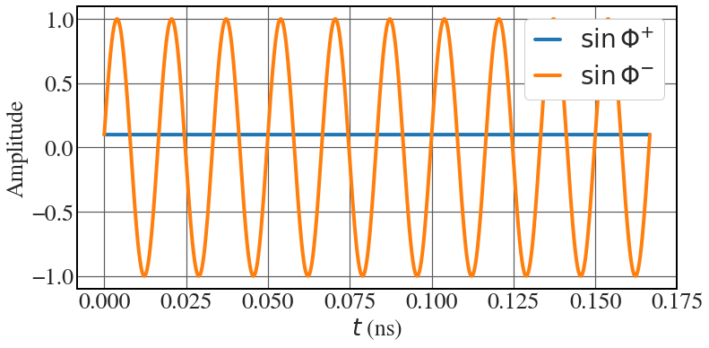
Ponderomotive phase
See Fig. 8.7.
|
1 2 3 4 5 6 7 8 9 10 11 12 13 14 15 16 17 18 19 20 |
Phi_pos = -0.1 lambda_u = 0.01 k_u = 2*np.pi/lambda_u c = 3.0e8 omega_u = 2*k_u*c print(1e-11*omega_u) N = 10 t = np.linspace(0,N*2*np.pi/omega_u,1000000) with plt.style.context(('seaborn-v0_8-whitegrid')): plt.rcParams.update(synchrotron_style) fig, ax = plt.subplots(figsize=(12,5.8)) ax.plot(1e9*t, -np.ones_like(t)*np.sin(Phi_pos), lw = 4, label="$\\sin \\Phi^{+}$") ax.plot(1e9*t, -np.sin(Phi_pos-omega_u*t), lw = 4, label="$\\sin \\Phi^{-}$") ax.tick_params(axis='y', labelsize=26) ax.tick_params(axis='x', labelsize=26) ax.set_ylabel('Amplitude', fontsize=26) ax.set_xlabel('$t$ (ns)', fontsize=26) ax.legend(fontsize=28, frameon=True, framealpha=1, handlelength=1) |
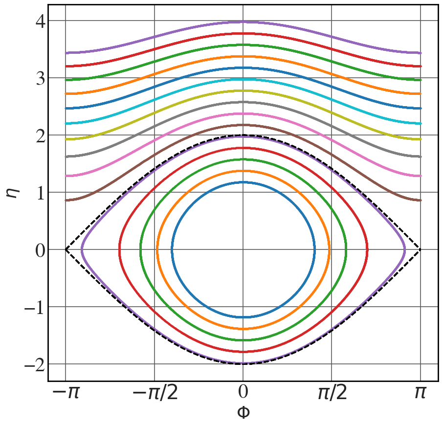
Numerical solution of the pendulum equation
See Fig. 8.8.
|
1 2 3 4 5 6 7 8 9 10 11 12 13 14 15 16 17 18 19 20 21 22 23 24 25 26 27 28 29 30 31 32 33 34 35 36 37 38 39 40 41 42 |
def system(initial_conditions, t, Omega_sq): # Set the initial conditions Phi = initial_conditions[0] eta = initial_conditions[1] # Write the coupled equations d_Phi = eta d_eta = -Omega_sq *np.sin(Phi) d_next_step = [d_Phi, d_eta] return d_next_step t = np.linspace(0,14.1,5000) eta0 = np.arange(1.18,4.18, 0.2) Omega_sq=1 Phi_sep = np.linspace(-np.pi,np.pi,256) eta_sep = np.sqrt(2*Omega_sq*(np.cos(Phi_sep)+1)) with plt.style.context(('seaborn-v0_8-whitegrid')): plt.rcParams.update(synchrotron_style) fig, ax = plt.subplots(figsize=(10.3,10)) for i in eta0: # Solve the system for different initial conditions initial_conditions = [0,i] final_conditions = odeint(system,initial_conditions, t, args=(Omega_sq,) ) ax.scatter((final_conditions[:,0]+np.pi)%(2*np.pi) - np.pi, final_conditions[:,1], s=3) ax.plot(Phi_sep, eta_sep, 'k--', lw=2) ax.plot(Phi_sep, -eta_sep, 'k--', lw=2) ax.set_xticks([-np.pi, -np.pi/2, 0, np.pi/2, np.pi]) ax.set_xticklabels(["$-\pi$", "$-\pi/2$", "0", "$\pi/2$", "$\pi$"], fontsize=16) ax.set_xlabel("$\\Phi$",fontsize=26) ax.set_ylabel("$\\eta$",fontsize=26) ax.tick_params(axis='y', labelsize=30) ax.tick_params(axis='x', labelsize=30) plt.show() |
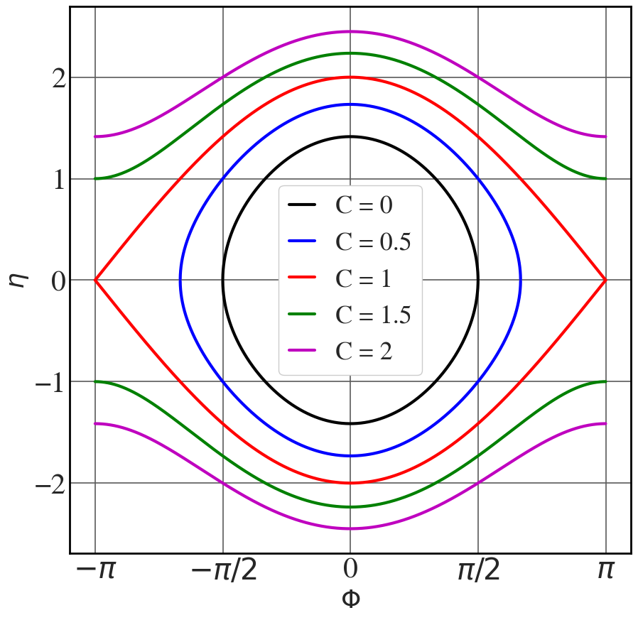
Phase-space trajectories
See Fig. 8.9.
|
1 2 3 4 5 6 7 8 9 10 11 12 13 14 15 16 17 18 19 20 21 22 23 24 |
Phi = np.linspace(-np.pi,np.pi,65536) Omega_sq=1 line_colour = ["k", "b", "r", "g", "m"] with plt.style.context(('seaborn-v0_8-whitegrid')): plt.rcParams.update(synchrotron_style) fig, ax = plt.subplots(figsize=(10.2,10)) for i, C in enumerate([0,0.5,1,1.5,2]): eta = np.sqrt(2*Omega_sq*(np.cos(Phi)+C)) ax.plot(Phi, eta, color = line_colour[i], lw=3) ax.plot(Phi, -eta, color = line_colour[i], lw=3, label="C = "+str(C)) ax.set_xticks([-np.pi, -np.pi/2, 0, np.pi/2, np.pi]) ax.set_xticklabels(["$-\pi$", "$-\pi/2$", "0", "$\pi/2$", "$\pi$"], fontsize=16) ax.set_xlabel("$\\Phi$",fontsize=26) ax.set_ylabel("$\\eta$",fontsize=26) ax.tick_params(axis='y', labelsize=30) ax.tick_params(axis='x', labelsize=30 ) plt.legend(fontsize=26, frameon=True, framealpha=1, handlelength=1) plt.show() |
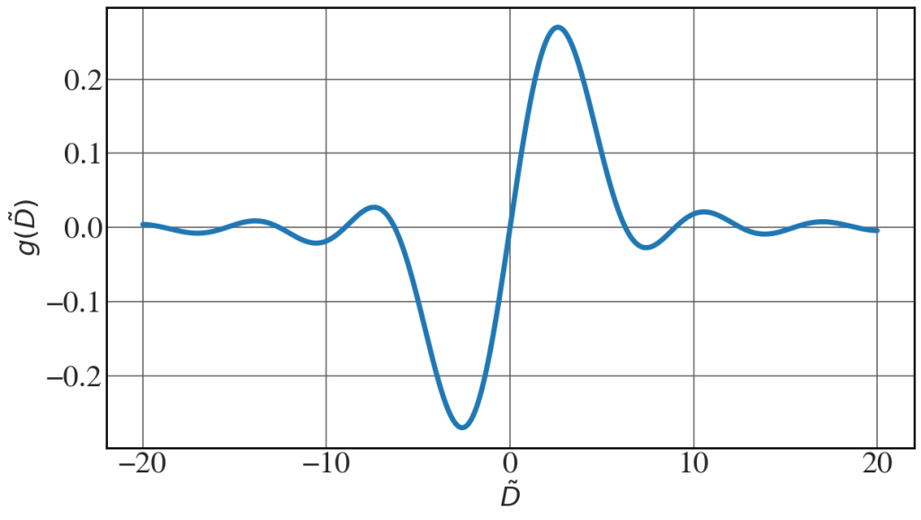
Plot of the gain function
See Fig. 8.10.
|
1 2 3 4 5 6 7 8 9 10 11 12 13 |
det = np.linspace(-20,20,2000) #detuning parameter gain = (4/det**3)*(1 - np.cos(det)- 0.5*det*np.sin(det)) with plt.style.context(('seaborn-whitegrid')): plt.rcParams.update(synchrotron_style) fig, ax = plt.subplots(figsize=(14,7.7)) ax.plot(det, gain, lw=5) ax.set_xlabel("$\\tilde{D}$",fontsize=26) ax.set_ylabel("$g(\\tilde{D})$",fontsize=26) ax.tick_params(axis='y', labelsize=30) ax.tick_params(axis='x', labelsize=30) plt.show() |
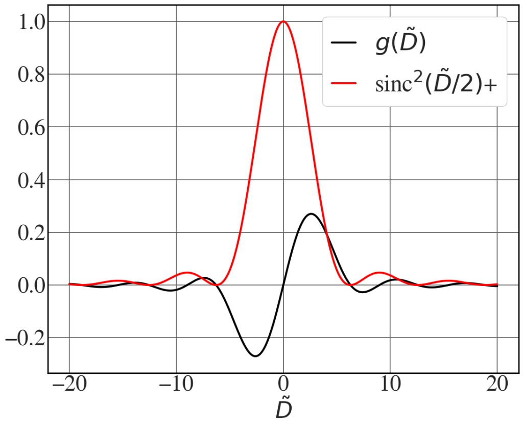
Gain and line width: Madey’s theorem
See Fig. 8.11.
|
1 2 3 4 5 6 7 8 9 10 11 12 13 14 15 16 |
det = np.linspace(-20,20,2000) #detuning parameter gain = (4/det**3)*(1 - np.cos(det)- 0.5*det*np.sin(det)) with plt.style.context(('seaborn-whitegrid')): plt.rcParams.update(synchrotron_style) fig, ax = plt.subplots(figsize=(12.7,10)) ax.plot(det, gain, 'k',lw=3, label = '$g(\\tilde{D})$') ax.plot(det, (np.sin(det/2) / (det/2))**2, 'r', lw=3, label = 'sinc$^{2}(\\tilde{D}/2)$+') ax.set_xlabel("$\\tilde{D}$",fontsize=34) ax.tick_params(axis='y', labelsize=34) ax.tick_params(axis='x', labelsize=34) ax.legend(fontsize=36, loc=1, frameon=True, framealpha=1, handlelength=1) plt.show() |
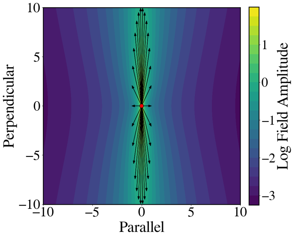
Relativistic length contraction of electric field lines
See Fig. 8.12.
First we define a function to calculate electric field components along two Cartesian coordinates.
|
1 2 3 4 5 6 7 8 9 10 11 12 |
def E(q,r_0, x,y, gamma): ''' Calculate components of Coulomb field''' eps_0 = 8.8541878188e-12 bet = np.sqrt(1-gamma**(-2)) r = np.hypot(x-r_0[0], y-r_0[1]) den = gamma**2 * r**3* (1-bet**2 * (y/r)**2)**1.5 E_x = q * (x - r_0[0]) / ((4*np.pi*eps_0)*den) E_y = q * (y - r_0[1]) / ((4*np.pi*eps_0)*den) return E_x, E_y |
Figure 8.12(b) can be generated using the code below. To generate Fig. 8.12(a), set the value of \gamma to 1.
|
1 2 3 4 5 6 7 8 9 10 11 12 13 14 15 16 17 18 19 20 21 22 23 24 25 26 27 28 29 30 31 32 33 34 35 36 37 38 39 40 41 42 43 44 45 46 47 48 49 50 |
# Define coordinates on a grid nx, ny = 128, 128 limit = 10 x = np.linspace(-limit, limit, nx) y = np.linspace(-limit, limit, ny) X, Y = np.meshgrid(x, y) # Generate field q = 1e-9 position = [0,0] gamma=10 Ex, Ey = E(q, position,x=X,y=Y, gamma=gamma) with plt.style.context(('default')): plt.rcParams.update(synchrotron_style) fig = plt.figure(figsize=(10,10)) ax = fig.add_subplot(111) # First generate the contour plot cp = ax.contourf(X, Y, np.log10(np.hypot(Ex, Ey)), levels=20, cmap=plt.cm.viridis) # Then add field lines for theta in np.linspace(0, 2*np.pi,30, endpoint=False): ax.arrow(0, 0, 10*np.cos(theta)/gamma, 10*np.sin(theta), head_width=0.2, length_includes_head=True, fc='k') # Add a dot at the position of the charge ax.add_artist(Circle(position, 0.02*limit, facecolor='red', edgecolor='black', zorder=10)) # Set limits and aspect ratio ax.set_xlim(-limit,limit) ax.set_ylim(-limit,limit) ax.set_aspect('equal') # Add a colorbar and scale its size to match the chart size cbar = fig.colorbar(cp, ax=ax, fraction=0.046, pad=0.04) cbar_ticks = np.arange(np.round(np.log10(np.hypot(Ex, Ey)).min()), np.round(np.log10(np.hypot(Ex, Ey)).max()),1) cbar.ax.set_yticks(cbar_ticks) cbar.ax.tick_params(axis='y', labelsize=34) ax.set_xlabel('Parallel', fontsize=40) ax.set_ylabel('Perpendicular', fontsize=40) cbar.ax.set_ylabel('Log Field Amplitude', fontsize=40) ax.set_xticks([-10,-5,0,5,10]) ax.set_yticks([-10,-5,0,5,10]) ax.tick_params(axis='x', labelsize=36) ax.tick_params(axis='y', labelsize=36) plt.show() |
High-gain simulations
The code to generate the high-gain simulation results in Figs. 8.14, 8.15, and 8.19 is longer than what it would fit in a single snippet. The entire Python script can be downloaded here.
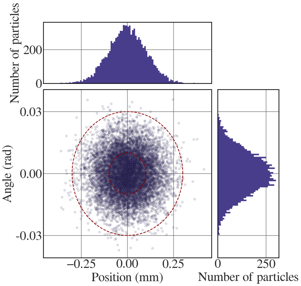
Beam emittance
The following code generates the distribution in Fig. 8.18(b).
|
1 2 3 4 5 6 7 8 9 10 11 12 13 14 15 16 17 18 19 20 21 22 23 24 25 26 27 28 29 30 31 32 33 34 35 36 37 38 39 40 41 42 43 44 45 46 47 48 49 50 51 52 53 54 55 56 57 58 59 60 61 62 63 64 65 66 67 68 69 70 71 |
# Generate a phase-sapce distribution of representative points n_p = 10000 mu_x, sigma_x = 0, 0.1 # mean and standard deviation of position mu_xp, sigma_xp = 0, 0.01 # mean and standard deviation of angle sx1 = np.random.normal(mu_x, sigma_x, n_p) sxp = np.random.normal(mu_xp, sigma_xp, n_p) sx2 = sx1 + 10*np.tan(sxp) def scatter_hist(x, y, ax, ax_histx, ax_histy): ax_histx.tick_params(axis="x", labelbottom=False) ax_histy.tick_params(axis="y", labelleft=False) # the scatter plot: ax.scatter(x, y, c='darkslateblue', edgecolors='k', alpha=0.15) # now determine nice limits by hand: nbins = 100 xmax = np.max(np.abs(x)) ymax = np.max(np.abs(y)) binwidthx = 2*xmax/nbins binwidthy = 2*ymax/nbins binsx = np.arange(-xmax, xmax + binwidthx, binwidthx) binsy = np.arange(-ymax, ymax + binwidthy, binwidthy) ax_histx.hist(x, bins=binsx, color='darkslateblue') ax_histy.hist(y, bins=binsy, color='darkslateblue', orientation='horizontal') ax_histx.set_ylabel('Number of particles') ax_histx.yaxis.label.set_fontsize(36) ax_histx.tick_params(axis='y', labelsize=36) ax_histy.set_xlabel('Number of particles') ax_histy.xaxis.label.set_fontsize(36) ax_histy.tick_params(axis='x', labelsize=36) ax.set_xlabel('Position (mm)') ax.set_ylabel('Angle (rad)') ax.xaxis.label.set_fontsize(36) ax.tick_params(axis='x', labelsize=36) ax.set_yticks([-0.03,0,0.03], ["-0.03","0.00","0.03"]) # ax.set_xticks([-0.3,0,0.3], ["-0.3","0.0","0.3"]) ax.yaxis.label.set_fontsize(36) ax.tick_params(axis='y', labelsize=36) # definitions for the axes left, width = 0.1, 0.55 bottom, height = 0.1, 0.55 spacing = 0.02 rect_scatter = [left, bottom, width, height] rect_histx = [left, bottom + height + spacing, width, 0.2] rect_histy = [left + width + spacing, bottom, 0.2, height] with plt.style.context(('seaborn-whitegrid')): plt.rcParams.update(synchrotron_style) fig = plt.figure(figsize=(12, 12)) ax = fig.add_axes(rect_scatter) ax_histx = fig.add_axes(rect_histx, sharex=ax) ax_histy = fig.add_axes(rect_histy, sharey=ax) # use the previously defined function scatter_hist(sx1, sxp, ax, ax_histx, ax_histy) t = np.linspace(0, 2*np.pi, 100) ax.plot(sigma_x*np.cos(t) , sigma_xp*np.sin(t), color='darkred', lw=2, ls = '--') ax.plot(3*sigma_x*np.cos(t) , 3*sigma_xp*np.sin(t), color='darkred', lw=2, ls = '--') plt.show() |
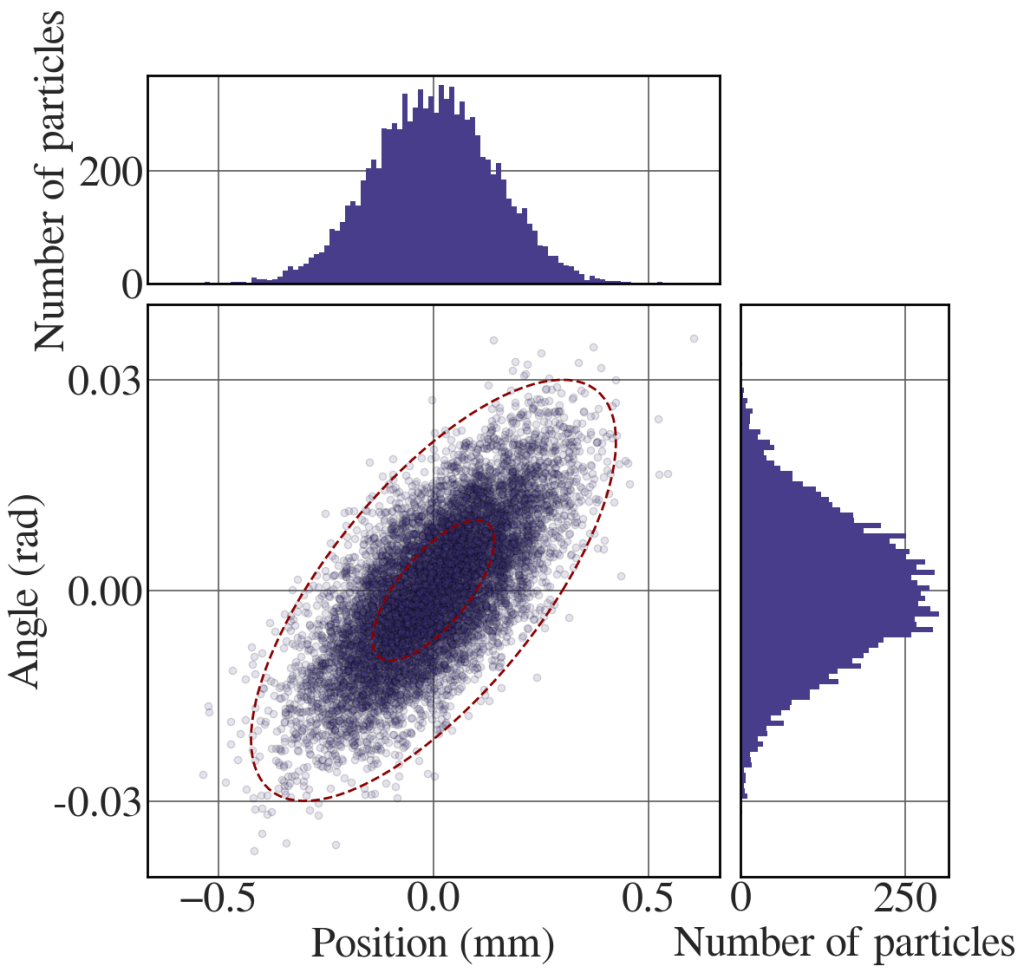
The following code generates the distribution in Fig. 8.18(c).
|
1 2 3 4 5 6 7 8 9 10 11 12 13 14 15 16 17 18 19 20 21 22 23 24 25 26 27 |
# Generate the same representative points after propagation # definitions for the axes left, width = 0.1, 0.55 bottom, height = 0.1, 0.55 spacing = 0.02 rect_scatter = [left, bottom, width, height] rect_histx = [left, bottom + height + spacing, width, 0.2] rect_histy = [left + width + spacing, bottom, 0.2, height] with plt.style.context(('seaborn-whitegrid')): plt.rcParams.update(synchrotron_style) fig = plt.figure(figsize=(12, 12)) ax = fig.add_axes(rect_scatter) ax_histx = fig.add_axes(rect_histx, sharex=ax) ax_histy = fig.add_axes(rect_histy, sharey=ax) # use the previously defined function scatter_hist(sx2, sxp, ax, ax_histx, ax_histy) t = np.linspace(0, 2*np.pi, 100) ax.plot(sigma_x*np.cos(t) + 10*sigma_xp*np.sin(t) , sigma_xp*np.sin(t), color='darkred', lw=2, ls = '--') ax.plot(3*sigma_x*np.cos(t) + 30*sigma_xp*np.sin(t) , 3*sigma_xp*np.sin(t), color='darkred', lw=2, ls = '--') plt.show() |
Bakers’ transformation
Figure 8.21 is generated using this Python script.
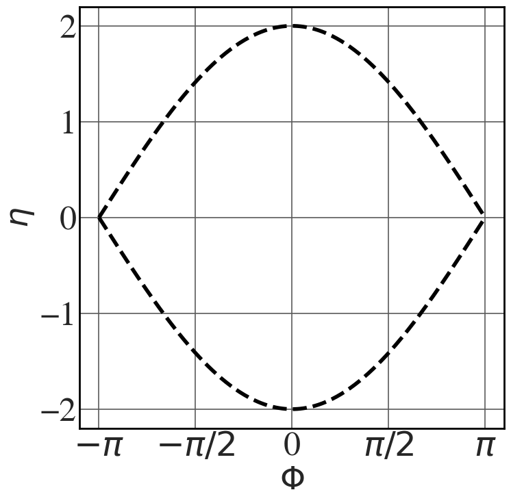
Separatrix
See Fig. 8.22.
|
1 2 3 4 5 6 7 8 9 10 11 12 13 14 15 16 17 18 19 20 21 22 |
t = np.linspace(0,10.1,5000) eta0 = [0.2] Omega_sq=1 Phi_sep = np.linspace(-np.pi,np.pi,256) eta_sep = np.sqrt(2*Omega_sq*(np.cos(Phi_sep)+1)) with plt.style.context(('seaborn-v0_8-whitegrid')): plt.rcParams.update(synchrotron_style) fig, ax = plt.subplots(figsize=(8,8)) for i in eta0: ax.plot(Phi_sep, eta_sep, 'k--', lw=4) ax.plot(Phi_sep, -eta_sep, 'k--', lw=4) ax.set_xticks([-np.pi, -np.pi/2, 0, np.pi/2, np.pi]) ax.set_xticklabels(["$-\pi$", "$-\pi/2$", "0", "$\pi/2$", "$\pi$"], fontsize=22) ax.set_xlabel("$\\Phi$",fontsize=34) ax.set_ylabel("$\\eta$",fontsize=34) ax.tick_params(axis='y', labelsize=36) ax.tick_params(axis='x', labelsize=36) |
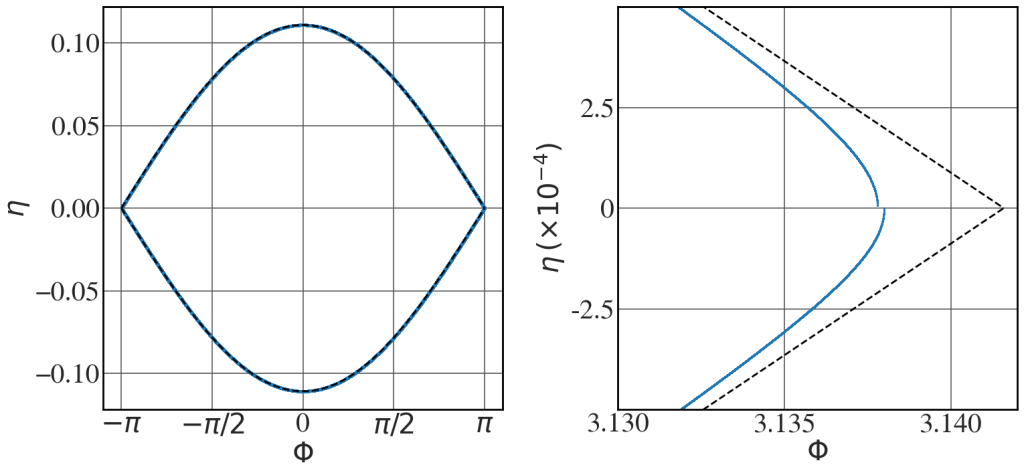
Solution of eqn (8.57)
See Fig. 8.24.
|
1 2 3 4 5 6 7 8 9 10 11 12 13 14 15 16 17 18 19 20 21 22 23 24 25 26 27 28 29 30 31 32 33 34 35 36 37 38 39 40 41 42 43 44 45 46 47 48 49 50 51 52 53 54 55 56 57 58 59 60 61 62 63 64 65 66 67 68 69 70 71 72 73 |
def pendulum(initial_conditions, t, Omega_sq): # Set the initial conditions Phi = initial_conditions[0] eta = initial_conditions[1] # Write the coupled equations d_Phi = eta d_eta = -Omega_sq *np.sin(Phi) d_next_step = [d_Phi, d_eta] return d_next_step mu_0 = 1.25663706212e-6 c = 3e8 gamma_r = 1000 K = 0.1 l_u = 0.1 k_u = 2*np.pi/l_u ee = 1.602176634e-19 me = 9.1093837015e-31 lambda_L = 1e-9 omega_L = 2*np.pi*c/lambda_L E_0 = 5e8 os = (ee*k_u*K*E_0)/(2*me*c**2*gamma_r**2) t = np.linspace(0,555.5,5000000) eps = 1.e-6 eta0 = [(1-eps)*2*np.sqrt(os)] print(eta0) Omega_sq=os initial_conditions = [3.138,0] final_conditions = odeint(pendulum,initial_conditions, t, args=(Omega_sq,) ) Phi_sep = np.linspace(-np.pi,np.pi,256) eta_sep = np.sqrt(2*Omega_sq*(np.cos(Phi_sep)+1)) with plt.style.context(('seaborn-v0_8-whitegrid')): plt.rcParams.update(synchrotron_style) fig, ax = plt.subplots(1,2, figsize=(16,7.8)) # for i in eta0: #initial_conditions = [0,i] ax[0].scatter((final_conditions[:,0]+np.pi)%(2*np.pi) - np.pi, final_conditions[:,1], s=3) ax[0].plot(Phi_sep, eta_sep, 'k--', lw=2) ax[0].plot(Phi_sep, -eta_sep, 'k--', lw=2) ax[1].scatter((final_conditions[:,0]+np.pi)%(2*np.pi) - np.pi, final_conditions[:,1], s=1) ax[1].plot(Phi_sep, eta_sep, 'k--', lw=2) ax[1].plot(Phi_sep, -eta_sep, 'k--', lw=2) ax[1].set_xlim(3.13,3.142) ax[1].set_ylim(-0.0005,0.0005) ax[0].set_xticks([-np.pi, -np.pi/2, 0, np.pi/2, np.pi]) ax[0].set_xticklabels(["$-\pi$", "$-\pi/2$", "0", "$\pi/2$", "$\pi$"], fontsize=16) ax[0].set_xlabel("$\\Phi$",fontsize=30) ax[0].set_ylabel("$\\eta$",fontsize=30) ax[0].tick_params(axis='y', labelsize=30) ax[0].tick_params(axis='x', labelsize=30) ax[1].set_yticks([-0.00025, 0, 0.00025]) ax[1].set_yticklabels(["-2.5", "0", "2.5"], fontsize=30) ax[1].set_xlabel("$\\Phi$",fontsize=30) ax[1].set_ylabel("$\\eta \\, (\\times 10^{-4})$",fontsize=30) ax[1].tick_params(axis='y', labelsize=30) ax[1].tick_params(axis='x', labelsize=30) plt.tight_layout() |
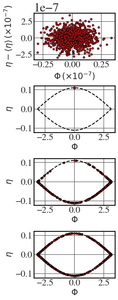
Laminar filamentation
See Fig. 8.23. The constants required in this code block are defined in the previous block.
|
1 2 3 4 5 6 7 8 9 10 11 12 13 14 15 16 17 18 19 20 21 22 23 24 25 26 27 28 29 30 31 32 33 34 35 36 37 38 39 40 41 42 43 44 45 46 47 |
eps=1e-5 t = np.linspace(0,50000.1,5000) n_p = 1000 eta_0 = 0.01*eps*np.random.randn(n_p) + (1-eps)*2*np.sqrt(os) phi_0 = 0.01*eps*np.random.randn(n_p) eta = np.zeros((t.shape[0], n_p)) phi = np.zeros((t.shape[0], n_p)) for i,j in enumerate(eta_0): initial_conditions = [phi_0[i],j] final_conditions = odeint(pendulum,initial_conditions, t, args=(os,) ) phi[:,i] = final_conditions[:,0] eta[:,i] = final_conditions[:,1] Phi_sep = np.linspace(-np.pi,np.pi,256) eta_sep = np.sqrt(2*Omega_sq*(np.cos(Phi_sep)+1)) time_intervals = np.linspace(0,500000,65)#[:-2] colour = 'red' #'darkslateblue' with plt.style.context(('seaborn-v0_8-whitegrid')): plt.rcParams.update(synchrotron_style) fig, axs = plt.subplots(4,1, figsize=(4,10)) axs[0].scatter(1e6*phi[0,:], eta[0,:]-eta[0,:].mean(), s=20, c=colour, ec='k') axs[1].scatter(phi[0,:], eta[0,:], s=20, c=colour, ec='k') axs[2].scatter(phi[2500,:], eta[2500,:], s=20, c=colour, ec='k') axs[3].scatter(phi[-1,:], eta[-1:], s=20, c=colour, ec='k') for idx, ax in enumerate(axs.flat): if idx !=0: ax.plot(Phi_sep, eta_sep, 'k--', lw=2) ax.plot(Phi_sep, -eta_sep, 'k--', lw=2) if idx ==0: ax.set_xlabel("$\\Phi \\, (\\times 10^{-7})$",fontsize=20) ax.set_ylabel("$\\eta - \\langle \\eta \\rangle \\, (\\times 10^{-7})$",fontsize=20) ax.tick_params(axis='y', labelsize=22) ax.tick_params(axis='x', labelsize=22) else: ax.set_xlabel("$\\Phi$",fontsize=20) ax.set_ylabel("$\\eta$",fontsize=20) ax.tick_params(axis='y', labelsize=22) ax.tick_params(axis='x', labelsize=22) plt.tight_layout() |
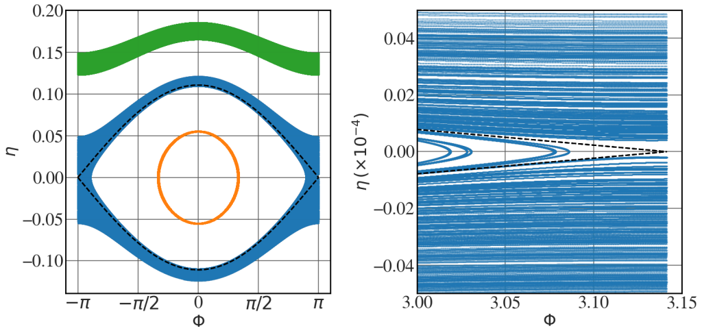
Stochastic layer
See Fig. 8.25.
|
1 2 3 4 5 6 7 8 9 10 11 12 13 14 15 16 17 18 19 20 21 22 23 24 25 26 27 28 29 30 31 32 33 34 35 36 37 38 39 40 41 42 43 44 45 46 47 48 49 50 51 52 53 54 55 56 57 58 59 60 61 62 63 64 65 66 67 68 69 70 71 |
def pendulum_perturbation(initial_conditions, t, Omega_sq, epsilon, omega_0): # Set the initial conditions Phi = initial_conditions[0] eta = initial_conditions[1] # Write the coupled equations d_Phi = eta d_eta = -Omega_sq *np.sin(Phi) + epsilon*Omega_sq *np.sin(omega_0*t) d_next_step = [d_Phi, d_eta] return d_next_step mu_0 = 1.25663706212e-6 c = 3e8 gamma_r = 1000 K = 0.1 l_u = 0.1 k_u = 2*np.pi/l_u ee = 1.602176634e-19 me = 9.1093837015e-31 lambda_L = 1e-9 omega_L = 2*np.pi*c/lambda_L E_0 = 5e8 os = (ee*k_u*K*E_0)/(2*me*c**2*gamma_r**2) omega_0=0.9*os t = np.linspace(0,50000,5000000) eps = 2.e-3 eta0 = [(1-eps)*2*np.sqrt(os), 0.5*(1-eps)*2*np.sqrt(os), 1.5*(1-eps)*2*np.sqrt(os)]#[0.11081005] print(eta0) Omega_sq=os epsilon=0.01 Phi_sep = np.linspace(-np.pi,np.pi,256) eta_sep = np.sqrt(2*Omega_sq*(np.cos(Phi_sep)+1)) with plt.style.context(('seaborn-v0_8-whitegrid')): plt.rcParams.update(synchrotron_style) fig, ax = plt.subplots(1,2, figsize=(16,8)) for i,j in enumerate(eta0): initial_conditions = [0,j] final_conditions = odeint(pendulum_perturbation,initial_conditions, t, args=(Omega_sq,epsilon, omega_0) ) ax[0].scatter((final_conditions[:,0]+np.pi)%(2*np.pi) - np.pi, final_conditions[:,1], s=2, alpha=0.25) ax[0].plot(Phi_sep, eta_sep, 'k--', lw=2) ax[0].plot(Phi_sep, -eta_sep, 'k--', lw=2) ax[1].scatter((final_conditions[:,0]+np.pi)%(2*np.pi) - np.pi, final_conditions[:,1], s=2, alpha=0.25) ax[1].plot(Phi_sep, eta_sep, 'k--', lw=2) ax[1].plot(Phi_sep, -eta_sep, 'k--', lw=2) ax[1].set_xlim(3,3.15) ax[1].set_ylim(-0.05,0.05) ax[0].set_xticks([-np.pi, -np.pi/2, 0, np.pi/2, np.pi]) ax[0].set_xticklabels(["$-\pi$", "$-\pi/2$", "0", "$\pi/2$", "$\pi$"], fontsize=16) ax[0].set_xlabel("$\\Phi$",fontsize=26) ax[0].set_ylabel("$\\eta$",fontsize=26) ax[0].tick_params(axis='y', labelsize=28) ax[0].tick_params(axis='x', labelsize=28) ax[1].set_xlabel("$\\Phi$",fontsize=26) ax[1].set_ylabel("$\\eta \\, (\\times 10^{-4})$",fontsize=26) ax[1].tick_params(axis='y', labelsize=28) ax[1].tick_params(axis='x', labelsize=28) plt.tight_layout() |
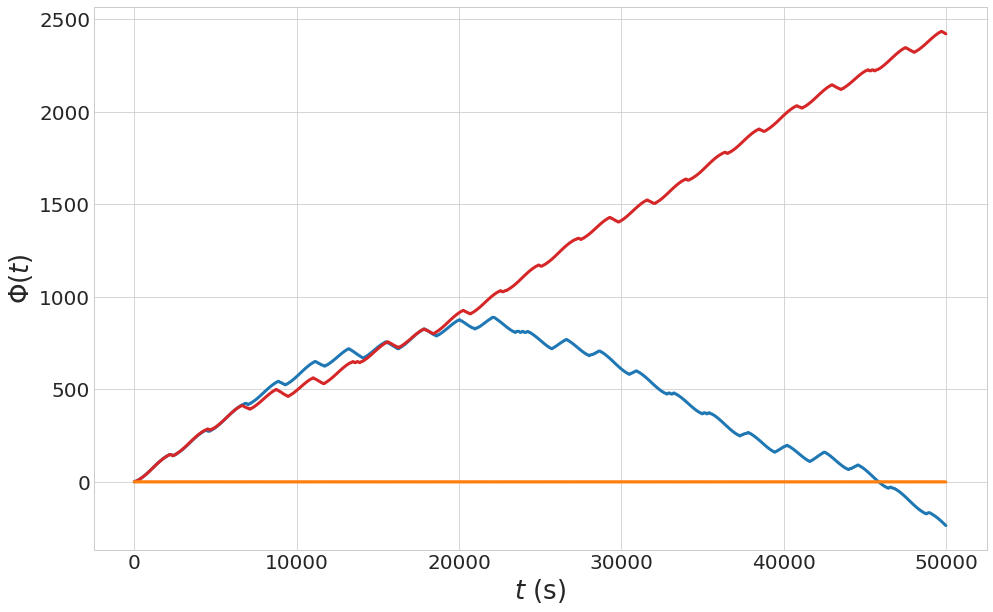
Turbulent chaotic evolution
See Fig. 8.26. The function “pendulum_perturbation” using in this block, has been defined in the previous block of code.
|
1 2 3 4 5 6 7 8 9 10 11 12 13 14 15 16 17 18 |
t = np.linspace(0,50000,1000000) epsilon=0.01 eta0 = [(1-eps)*2*np.sqrt(os), 0.9999*(1-eps)*2*np.sqrt(os), 0.5*(1-eps)*2*np.sqrt(os)] color = ['#1f77b4', '#d62728', '#ff7f0e'] omega_0=0.9*os with plt.style.context(('seaborn-whitegrid')): fig, ax = plt.subplots(figsize=(16,10)) for i,j in enumerate(eta0): initial_conditions = [0,j] final_conditions = odeint(pendulum_perturbation,initial_conditions, t, args=(Omega_sq,epsilon, omega_0) ) ax.plot(t[:],final_conditions[:,0], lw=3, color=color[i]) ax.set_xlabel("$t$ (s)",fontsize=26) ax.set_ylabel("$\\Phi (t)$",fontsize=26) ax.tick_params(axis='y', labelsize=20) ax.tick_params(axis='x', labelsize=20) plt.show() |