Below is a set of python codes associated with Chapter 2 of Daniele Pelliccia and David M. Paganin, “Synchrotron Light: A Physics Journey from Laboratory to Cosmos” (Oxford University Press, 2025).
In order to run any of these python codes, you will need to include the following header file.
|
1 2 3 4 5 6 7 8 9 10 11 12 |
import numpy as np import matplotlib.pyplot as plt from matplotlib.patches import Circle synchrotron_style = { 'font.family': 'FreeSerif', 'font.size': 30, 'axes.linewidth': 2.0, 'axes.edgecolor': 'black', 'grid.color': '#5b5b5b', 'grid.linewidth': 1.2, } |
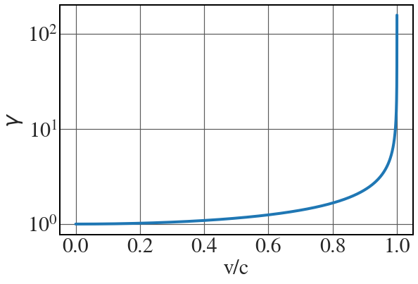
Plot of the Lorentz factor
See Fig. 2.7.
|
1 2 3 4 5 6 7 8 9 10 11 12 13 |
c = 1. # set the speed of light in natural units v = np.linspace(0, c, 50000, endpoint=False) # define an array containing the value of the velocity gamma = 1.0/ np.sqrt(1.0 - v**2/c**2) fig = plt.figure(figsize=(9,6)) with plt.style.context(('seaborn-v0_8-whitegrid')): plt.rcParams.update(synchrotron_style) plt.semilogy(v,gamma, lw=4) plt.xlabel('v/c', fontsize=30) plt.ylabel('$\gamma$', fontsize=30) plt.show() |
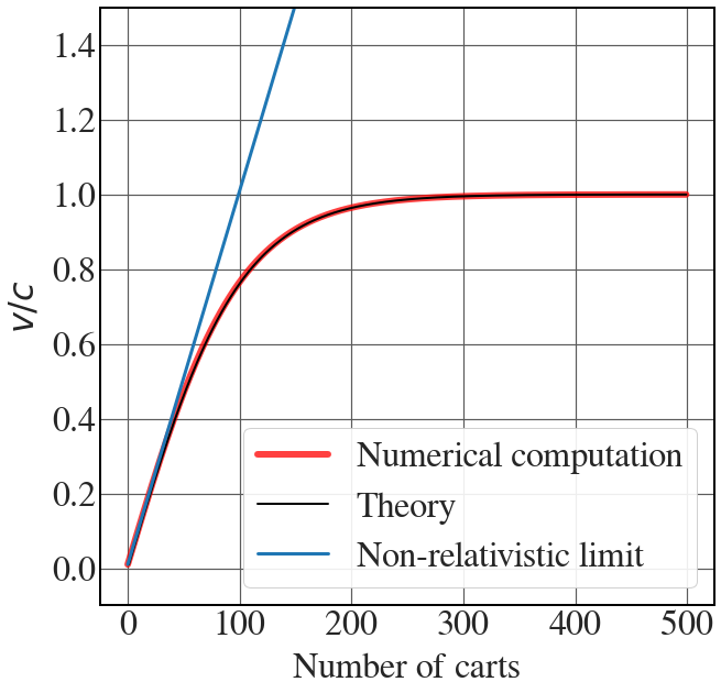
An infinity of stacked carts
See computational exercise on page 29, together with Figs. 2.14-2.15.
|
1 2 3 4 5 6 7 8 9 10 11 12 13 14 15 16 17 |
ncarts = 500 V = 0.01 # start with a velocity that is 1% of the speed of light v_th = np.zeros(ncarts) # Theory v_gal = np.zeros(ncarts) # Galileo transformation v_lor = np.zeros(ncarts) # Lorentz transformation # Set the first velocity to V v_th[0] = V v_gal[0] = V v_lor[0] = V for i in range(1,ncarts,1): v_th[i] = ( (1+v_th[0])**i - (1-v_th[0])**i ) / ( (1+v_th[0])**i + (1-v_th[0])**i ) v_lor[i] = (v_lor[i-1]+V) / (1+ v_lor[i-1]*V) v_gal[i] = v_gal[i-1]+V |
|
1 2 3 4 5 6 7 8 9 10 11 12 13 14 |
fig = plt.figure(figsize=(10,10)) with plt.style.context(('seaborn-v0_8-whitegrid')): plt.rcParams.update(synchrotron_style) plt.plot(v_lor, color='r', lw=6, alpha=0.75, label = 'Numerical computation') plt.plot(v_th, 'k', lw=2, label = 'Theory') plt.plot(v_gal, lw=3, label = 'Non-relativistic limit') plt.ylim(-0.1,1.5) plt.legend(fontsize = 32, frameon=True, loc = 'lower right', framealpha=0.9) plt.xticks(fontsize = 32) plt.yticks(fontsize = 32) plt.xlabel('Number of carts', fontsize=32, labelpad=10) plt.ylabel("$v/c$", rotation=90, fontsize=32, labelpad=10) plt.show() |
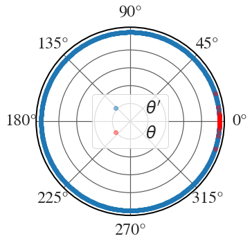
Relativistic aberration
See Fig. 2.17.
|
1 2 3 4 5 6 7 8 9 10 11 12 13 14 15 16 17 18 19 20 |
gamma = 1000 # Set gamma = 100 to generate Fig. 2.17(a) beta = np.sqrt(1-gamma**(-2)) thetap = np.linspace(0, 2*np.pi, 1000, endpoint=False) theta = np.arcsin( np.sin(thetap)/ (gamma*(1+beta*np.cos(thetap)) )) r = np.ones(thetap.shape[0]) with plt.style.context(('seaborn-v0_8-whitegrid')): plt.rcParams.update(synchrotron_style) fig = plt.figure(figsize=(5,5)) ax = fig.add_subplot(111, projection='polar') ax.plot(thetap, r, 'o', alpha=0.5, label="$\\theta'$") ax.plot(theta, r, 'o', ms = 6, markerfacecolor='r', markeredgecolor='r', alpha = 0.4, label="$\\theta$") # markeredgecolor='r' ax.set_yticklabels([]) ax.tick_params(axis='x', which='major', pad=15) plt.xticks(fontsize = 24) plt.legend(fontsize = 24, frameon=True) plt.show() |
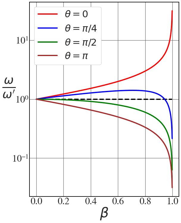
Longitudinal Doppler effect
See Fig. 2.20 for a plot of the dependency of the ratio \omega' / \omega as a function of the velocity, for four values of the direction angle \theta.
|
1 2 3 4 5 6 7 8 9 10 11 12 13 14 15 16 17 18 19 20 21 22 23 24 25 26 27 28 29 30 |
c = 1. # set the speed of light in natural units v = np.linspace(0, c, 500, endpoint=False) # define an array containing the value of the velocity beta = v/c gamma = 1.0/ np.sqrt(1.0 - v**2/c**2) theta1 = 0 theta2 = np.pi/4 theta3 = np.pi/2 theta4 = np.pi fig = plt.figure(figsize=(9,12)) with plt.style.context(('seaborn-v0_8-whitegrid')): plt.rcParams.update(synchrotron_style) plt.semilogy(beta, np.ones(beta.shape[0]), 'k--', lw =4) plt.semilogy(beta,1.0/(gamma*(1-beta*np.cos(theta1))), 'r', lw=4, label="$\\theta = 0$") plt.semilogy(beta,1.0/(gamma*(1-beta*np.cos(theta2))), 'b',lw=4, label="$\\theta = \pi/4$") plt.semilogy(beta,1.0/(gamma*(1-beta*np.cos(theta3))), 'g',lw=4, label="$\\theta = \pi/2$") plt.semilogy(beta,1.0/(gamma*(1-beta*np.cos(theta4))), 'brown',lw=4, label="$\\theta = \pi$") plt.xlabel('$\\beta$', fontsize=46, labelpad=0) plt.ylabel("$\\frac{\omega}{\omega'}$", rotation=0, fontsize=56, labelpad=10) plt.xticks(fontsize = 32) plt.yticks(fontsize = 32) plt.legend(fontsize = 32, frameon=True, framealpha=01.0) plt.show() |
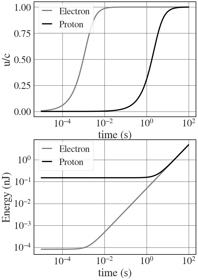
Acceleration of a particle pushed by a uniform force
See Figs. 2.23 and 2.24.
|
1 2 3 4 5 6 7 8 9 10 11 12 13 14 15 16 17 18 19 20 21 22 23 24 25 26 27 28 29 30 31 32 33 34 35 36 37 38 |
me = 9.109e-31 #kg mp = 1.673e-27 #kg e = 1.602e-19 #C c = 3.0e8 #m/s E = 1 #V/m t = np.logspace(-5, 2, 5000) # Define velocity as a dimensionless fraction of c ue = 1.0/np.sqrt(1+(me*c/(e*E*t))**2) up = 1.0/np.sqrt(1+(mp*c/(e*E*t))**2) gamma_e = 1.0/np.sqrt(1.-ue**2) gamma_p = 1.0/np.sqrt(1.-up**2) with plt.style.context(('seaborn-v0_8-whitegrid')): plt.rcParams.update(synchrotron_style) fig, axs = plt.subplots(2, 1,figsize=(10,16)) axs[0].semilogx(t, ue, 'grey', lw = 4, label = 'Electron') axs[0].semilogx(t, up, 'k', lw = 4, label = 'Proton') axs[1].loglog(t, gamma_e*me*c**2*1e9, 'grey', lw = 4, label = 'Electron') axs[1].loglog(t, gamma_p*mp*c**2*1e9, 'k', lw = 4, label = 'Proton') axs[0].tick_params(axis='both', which='major', labelsize=34, pad = 10) axs[1].tick_params(axis='both', which='major', labelsize=34, pad = 10) axs[0].set_xlabel('time (s)', fontsize=38) axs[1].set_xlabel('time (s)', fontsize=38) axs[0].set_ylabel('u/c', fontsize=38) axs[1].set_ylabel('Energy (nJ)', fontsize=38) axs[0].legend(fontsize = 32, frameon=True, loc='upper left', handlelength=1, bbox_to_anchor=(0.00001, 1.025)) axs[1].legend(fontsize = 32, frameon=True, loc='upper left', handlelength=1, bbox_to_anchor=(0.00001, 1.025)) plt.show() |
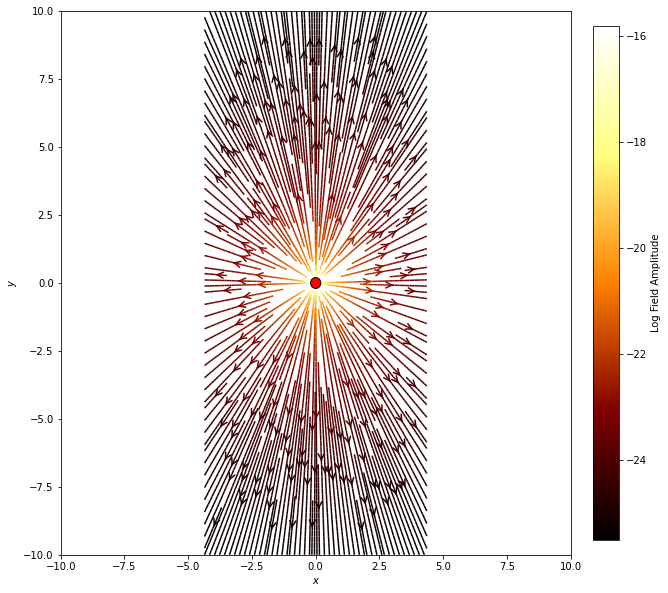
Bonus content: relativistic contraction of field lines
Let us suppose a charge is moving along the x-axis with constant speed v which is a sizeable fraction of the speed of light. How does the Coulomb field lines transform for an observer that is at rest compared to the moving charge? We expect the lines to be contracted by a factor \gamma in the direction of motion.
|
1 2 3 4 5 6 7 8 9 10 11 12 |
''' Define a function that generates the electric field components as a function of the charge q, position of the charge r_0 = (x_0, y_0), and the coordinate arrays x and y. To avoid potential numerical rounding errors with set 1/(4 pi epsilon_0) to be 1 ''' def E(q, x,y, gamma): den = np.hypot(x, y)**3 # denominator E_x = q * (x) / den E_y = q * (y) / den return E_x, E_y |
|
1 2 3 4 5 6 7 8 9 10 11 12 13 14 15 16 17 18 19 20 21 22 23 24 25 26 27 28 29 30 31 32 33 34 35 36 37 38 39 40 41 |
# Plot the field generated by a charge of 1 coulomb located at the origin beta = 0.9 gamma = (1.0-beta**2)**(-0.5) # Define coordinates on a grid nx, ny = 128, 128 limit = 10 x = np.linspace(-limit, limit, nx) y = np.linspace(-limit, limit, ny) X, Y = np.meshgrid(x/gamma, y) # Generate field q = 1e-9 position = [0,0] Ex, Ey = E(q, x=X,y=Y, gamma=gamma) fig = plt.figure(figsize=(10,10)) ax = fig.add_subplot(111) # Set the colour as the amplitude of the field. We take the log to ease the visualisation. color = np.log(np.hypot(Ex, Ey)) # Draw streamplot sp = ax.streamplot(X, Y, Ex, Ey, color=color, cmap=plt.cm.afmhot, \ density=3, arrowstyle='->', arrowsize=1.5) # Add a circle at the position of the charge. The command "zorder" forces the circle to be on top of the lines ax.add_artist(Circle(position, 0.02*limit, facecolor='red', edgecolor='black', zorder=10)) # Set limits and aspect ratio ax.set_xlim(-limit,limit) ax.set_ylim(-limit,limit) #ax.set_aspect('equal') # Add a colorbar and scale its size to match the chart size cbar = fig.colorbar(sp.lines, ax=ax, fraction=0.046, pad=0.04) ax.set_xlabel('$x$') ax.set_ylabel('$y$') cbar.ax.set_ylabel('Log Field Amplitude') plt.show() |