Below is a set of python codes associated with Chapter 4 of Daniele Pelliccia and David M. Paganin, “Synchrotron Light: A Physics Journey from Laboratory to Cosmos” (Oxford University Press, 2025).
In order to run any of these python codes, you will need to include the following header file.
|
1 2 3 4 5 6 7 8 9 10 11 12 13 14 15 16 |
import numpy as np import matplotlib.pyplot as plt from sys import stdout from mpl_toolkits.mplot3d import Axes3D from matplotlib import cm from matplotlib.colors import LightSource from scipy import special synchrotron_style = { 'font.family': 'FreeSerif', 'font.size': 30, 'axes.linewidth': 2.0, 'axes.edgecolor': 'black', 'grid.color': '#5b5b5b', 'grid.linewidth': 1.2, } |
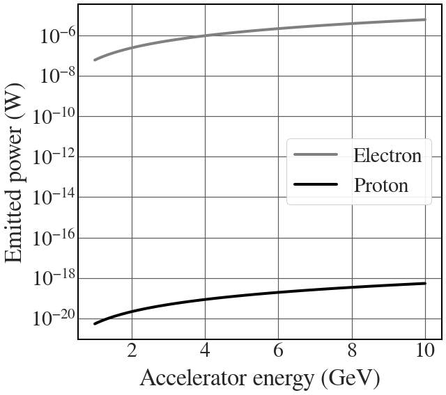
Synchrotron radiation for electrons and protons
See Fig. 4.2.
|
1 2 3 4 5 6 7 8 9 10 11 12 13 14 |
r_e = 2.817940323e-15 # m, classical electron radius e = 1.602176634e-19 # C, electron charge c = 2.99792458e8 # m/s, speed of light m_e = 9.109383702e-31 # kg, electron mass En_e = 0.510998950e-3 # GeV, electron rest energy. epsilon_0 = 8.854187813e-12 # F/m, vacuum permittivity m_p = 1.672621924e-27 # kg, proton mass r_p = 1.0/(4*np.pi*epsilon_0)*e**2/(m_p*c**2) #m, the equivalent of r_e for protons En_p = 0.93827208816 # GeV, proton rest energy # These constants are now in units of W T^{-2} GeV^{-2} C_e = (2/3)*(r_e*e**2*c/m_e)/En_e**2 C_p = (2/3)*(r_p*e**2*c/m_p)/En_p**2 |
|
1 2 3 4 5 6 7 8 9 10 11 12 13 14 15 16 17 18 19 |
B = 1.0 En = np.linspace(1, 10, 100) P_e = C_e*B**2*En**2 P_p = C_p*B**2*En**2 with plt.style.context(('seaborn-v0_8-whitegrid')): plt.rcParams.update(synchrotron_style) fig = plt.figure(figsize=(9,8)) plt.semilogy(En, P_e, 'grey', lw = 4, label="Electron") plt.semilogy(En, P_p, 'k', lw = 4, label="Proton") plt.legend(fontsize = 30, frameon=True, framealpha=0.9) plt.xticks(fontsize = 30) plt.yticks(fontsize = 30) plt.xlabel('Accelerator energy (GeV)', fontsize=34, labelpad=10) plt.ylabel("Emitted power (W)", fontsize=34, labelpad=5) plt.tight_layout() plt.show() |
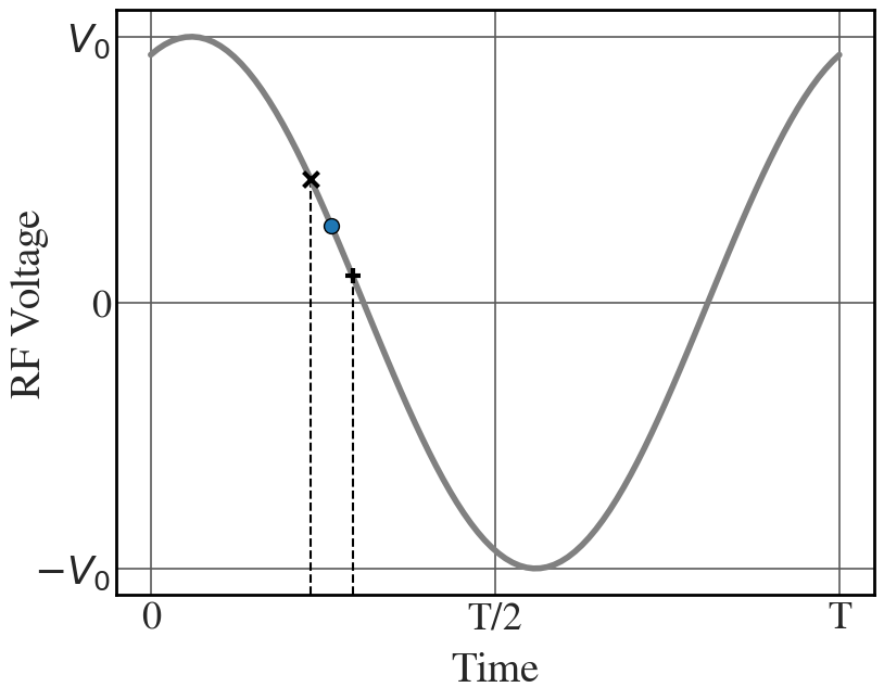
Radio-frequency cavity
See Fig. 4.4.
|
1 2 3 4 5 6 7 8 9 10 11 12 13 14 15 16 17 18 19 20 21 22 23 24 25 26 |
omega = 2*np.pi phi = 1.2 t = np.linspace(0, 1, 100) V = np.sin(omega*t+phi) with plt.style.context(('seaborn-v0_8-whitegrid')): plt.rcParams.update(synchrotron_style) fig = plt.figure(figsize=(9,7)) plt.plot(t, V, 'grey', lw = 4,zorder=2) plt.scatter(t[26],V[26], s = 100, edgecolors='black',zorder=3 ) plt.scatter(t[23],V[23], marker = 'x', s = 100, c='black',linewidths=3, zorder=3 ) plt.scatter(t[29],V[29], marker = '+', s = 100, c='black',linewidths=3, zorder=3 ) plt.plot([t[23], t[23]], [-1.1, V[23]], 'k--', zorder=1) plt.plot([t[29], t[29]], [-1.1, V[29]], 'k--', zorder=1) #plt.plot([t[26], t[26]], [-1.1, V[26]], 'k--', zorder=1) # plt.legend(fontsize = 24, frameon=True) plt.ylim(-1.1,1.1) plt.xticks([0.0, 0.5, 1.], ["0", "T/2", "T"], fontsize = 26) #plt.xticks(fontsize = 24) plt.yticks([-1, 0.0, 1.], ["$-V_{0}$", "0", "$V_{0}$"], fontsize = 26) plt.xlabel('Time', fontsize=28, labelpad=10) plt.ylabel("RF Voltage", fontsize=28, labelpad=-10) plt.show() |
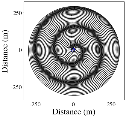
Simplified plot of synchrotron emission
The following code will generate one of the panels in Fig 4.8. Repeat the simulation by changing \beta.
|
1 2 3 4 5 6 7 8 9 10 11 12 13 14 15 16 17 18 19 20 21 22 23 24 25 26 27 28 29 30 |
c = 2.99792458e8 # m/s, speed of light beta = 0.5 rho = 10 omega_0 = beta*c/rho theta = np.linspace(0, 2*np.pi, 100, endpoint=True) t = np.linspace(0.000001,0, 50) with plt.style.context(('default')): plt.rcParams.update(synchrotron_style) fig = plt.figure(figsize=(6,6)) plt.plot(rho*np.cos(theta), rho*np.sin(theta), 'b', lw=2) for i,j in enumerate(t): cx = rho*np.cos(omega_0*j) cy = rho*np.sin(omega_0*j) a = cx + c*j*np.cos(theta) b = cy + c*j*np.sin(theta) plt.plot(b, a, 'k') plt.xlabel("Distance (m)", fontsize=28) plt.ylabel("Distance (m)", fontsize=28) plt.xticks(ticks = [-250, 0, 250],labels=("-250", "0", "250"), fontsize = 20) plt.yticks(ticks = [-250, 0, 250],labels=("-250", "0", "250"), fontsize = 20) plt.show() |
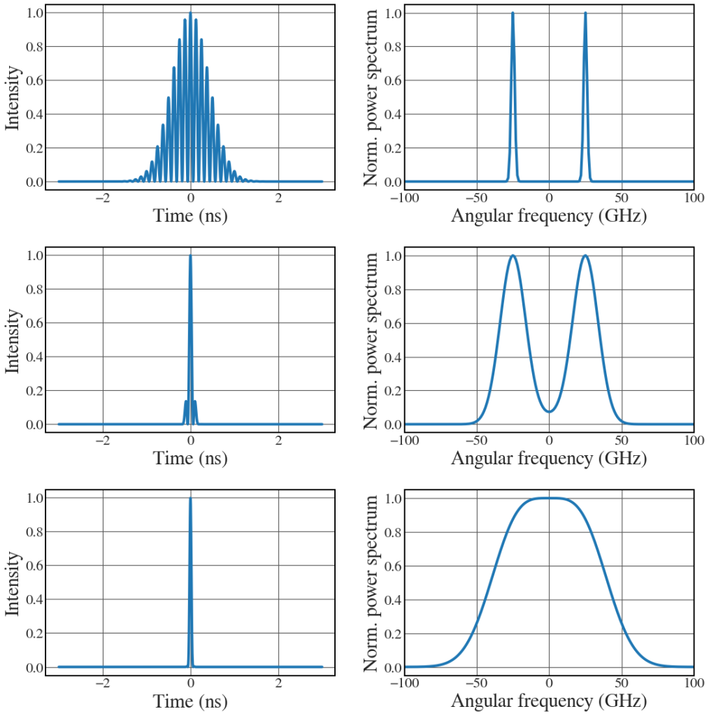
Time-bandwidth uncertainty relation
See Fig. 4.11.
|
1 2 3 4 5 6 7 8 9 10 11 12 13 14 15 16 17 18 19 20 21 22 23 24 25 26 27 28 29 30 31 32 33 34 35 36 37 38 39 40 41 42 43 44 45 46 47 48 49 50 51 52 53 54 55 56 57 58 59 60 61 62 63 64 65 66 67 68 69 70 71 72 73 74 75 76 77 |
n_points = 1500 # Time sequence t = np.linspace(-3, 3, n_points) # units of nanoseconds dt = t[2] - t[1] v_0 = 4 # Central frequency, 1/ns omega_0 = 25 # 2*np.pi*4 # Central frequency # Frequency sequence v = (1.0/ (n_points*dt))* (np.arange(n_points) - n_points//2) omega = (2*np.pi/ (n_points*dt))* (np.arange(n_points) - n_points//2) dv = v[1]-v[0] # Pulse duration delta_t1 = 0.6 #ns delta_t2 = 0.08 #ns delta_t3 = 0.04 #ns # Define pulse with Gaussian envelope pulse1 = np.cos(omega_0*t) * np.exp(-t**2/(2*delta_t1**2)) pulse2 = np.cos(omega_0*t) * np.exp(-t**2/(2*delta_t2**2)) pulse3 = np.cos(omega_0*t) * np.exp(-t**2/(2*delta_t3**2)) # Fourier Transform of the pulse f_p1 = np.fft.fftshift(np.fft.fft(pulse1))/np.sqrt(n_points) f_p2 = np.fft.fftshift(np.fft.fft(pulse2))/np.sqrt(n_points) f_p3 = np.fft.fftshift(np.fft.fft(pulse3))/np.sqrt(n_points) tick_size = 22 font_size = 30 with plt.style.context(('seaborn-v0_8-whitegrid')): plt.rcParams.update(synchrotron_style) fig, axs = plt.subplots(3,2, figsize=(16,16)) axs[0,0].plot(t, np.real(pulse1)**2, lw=4) axs[0,0].tick_params(axis='x', labelsize=tick_size) axs[0,0].tick_params(axis='y', labelsize=tick_size) axs[0,0].set_xlabel('Time (ns)', fontsize=font_size) axs[0,0].set_ylabel('Intensity', fontsize=font_size) ### axs[0,1].plot(omega, np.abs(f_p1)**2/(np.abs(f_p1)**2).max(), lw=4) axs[0,1].set_xlim([-100, 100]) axs[0,1].tick_params(axis='x', labelsize=tick_size) axs[0,1].tick_params(axis='y', labelsize=tick_size) axs[0,1].set_xlabel('Angular frequency (GHz)', fontsize=font_size) axs[0,1].set_ylabel('Norm. power spectrum', fontsize=font_size) axs[1,0].plot(t, np.real(pulse2)**2, lw=4) axs[1,0].tick_params(axis='x', labelsize=tick_size) axs[1,0].tick_params(axis='y', labelsize=tick_size) axs[1,0].set_xlabel('Time (ns)', fontsize=font_size) axs[1,0].set_ylabel('Intensity', fontsize=font_size) ### axs[1,1].plot(omega, np.abs(f_p2)**2/(np.abs(f_p2)**2).max(), lw=4) axs[1,1].set_xlim([-100, 100]) axs[1,1].tick_params(axis='x', labelsize=tick_size) axs[1,1].tick_params(axis='y', labelsize=tick_size) axs[1,1].set_xlabel('Angular frequency (GHz)', fontsize=font_size) axs[1,1].set_ylabel('Norm. power spectrum', fontsize=font_size) axs[2,0].plot(t, np.real(pulse3)**2, lw=4) axs[2,0].tick_params(axis='x', labelsize=tick_size) axs[2,0].tick_params(axis='y', labelsize=tick_size) axs[2,0].set_xlabel('Time (ns)', fontsize=font_size) axs[2,0].set_ylabel('Intensity', fontsize=font_size) ### axs[2,1].plot(omega, np.abs(f_p3)**2/(np.abs(f_p3)**2).max(), lw=4) axs[2,1].set_xlim([-100, 100]) axs[2,1].tick_params(axis='x', labelsize=tick_size) axs[2,1].tick_params(axis='y', labelsize=tick_size) axs[2,1].set_xlabel('Angular frequency (GHz)', fontsize=font_size) axs[2,1].set_ylabel('Norm. power spectrum', fontsize=font_size) plt.tight_layout() #w_pad=2 plt.show() |
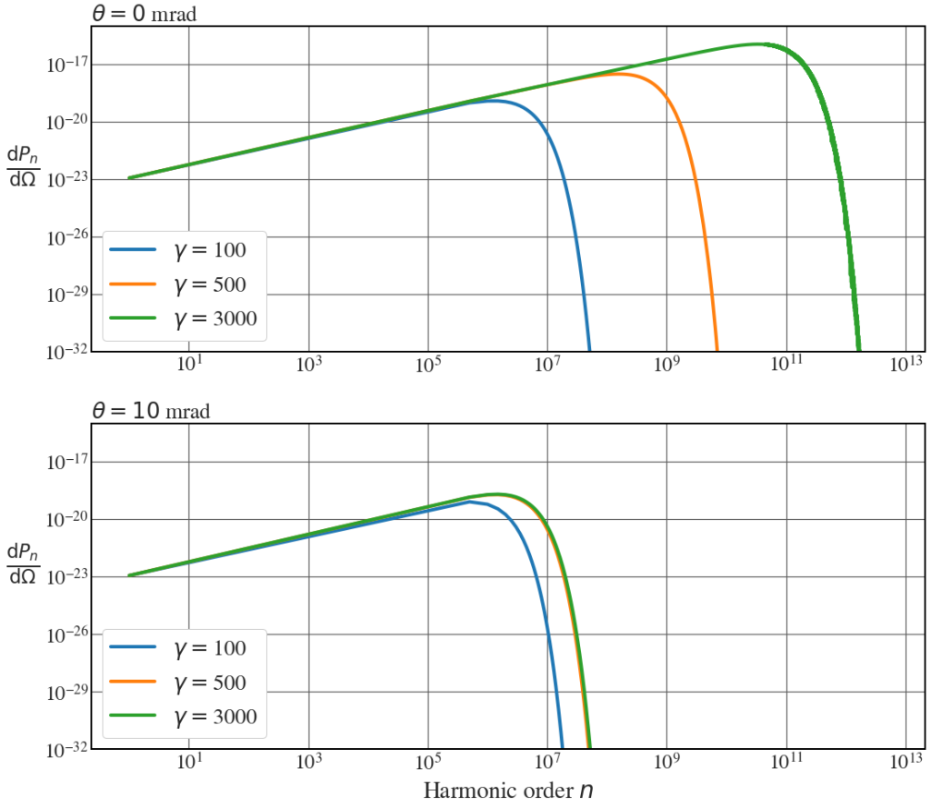
Spectral plots
Radiated power as a function of the harmonic order in Fig. 4.14.
|
1 2 3 4 5 6 7 8 9 10 11 12 13 14 15 16 17 18 19 20 21 22 23 24 25 26 27 28 29 30 31 32 33 34 35 36 37 38 39 40 41 42 43 44 45 46 |
e = 1.602e-19 #C c = 3.0e8 #m/s rho = 10 #m epsilon_0 = 8.854e-12 #F/m P_0 = (1.0/(8*np.pi**2*epsilon_0)) * (c*e**2 /(rho**2)) n = np.linspace(1,int(5e12), int(1e7)) with plt.style.context(('seaborn-v0_8-whitegrid')): plt.rcParams.update(synchrotron_style) fig, ax = plt.subplots(2,1, figsize=(16,14)) for th, theta in enumerate([0.0, 0.01]): for gamma in [100, 500, 3000]: beta = np.sqrt(1-1/gamma**2) power = P_0*n**2 *beta**4 *(special.jvp(n,n*beta*np.cos(theta))**2 + np.tan(theta)**2 * \ special.jv(n,n*beta*np.cos(theta))**2 / beta**2 ) ax[th].loglog(n, power, lw = 4, label="$\\gamma=$"+str(gamma)) print(power.max()/power[0]) ax[0].legend(fontsize = 26, frameon=True, loc='lower left', framealpha=1) ax[1].legend(fontsize = 26, frameon=True, loc='lower left', framealpha=1) ax[0].tick_params(axis='x', labelsize=24) ax[0].tick_params(axis='y', labelsize=24) ax[1].tick_params(axis='x', labelsize=24) ax[1].tick_params(axis='y', labelsize=24) plt.xlabel('Harmonic order $n$', fontsize=28, labelpad=10) ax[0].set_ylabel("$\\frac{\mathrm{d}P_{n}}{\mathrm{d}\Omega}$", rotation=0, fontsize=32, labelpad=25) ax[1].set_ylabel("$\\frac{\mathrm{d}P_{n}}{\mathrm{d}\Omega}$", rotation=0, fontsize=32, labelpad=25) ax[0].set_title("$\\theta=0$ mrad", fontsize = 26, loc='left') ax[1].set_title("$\\theta=10$ mrad", fontsize = 26, loc='left') ax[0].set_ylim([1e-32, 1e-15]) ax[1].set_ylim([1e-32, 1e-15]) plt.tight_layout() #h_pad=4 plt.show() |
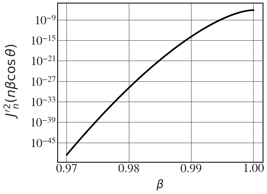
Plots of J_n^{2}(n \beta) and J_n^{'2}(n \beta) vs \beta
See Fig. 4.15.
|
1 2 3 4 5 6 7 8 9 10 11 |
beta = np.linspace(0.97,0.9999999, 1000) theta=0 nn = 10000 with plt.style.context(('seaborn-v0_8-whitegrid')): plt.rcParams.update(synchrotron_style) fig = plt.figure(figsize=(9,7)) plt.semilogy(beta, special.jvp(nn,nn*beta*np.cos(theta))**2, 'k', lw = 4, label="$\\beta=$"+str(beta)) plt.xlabel('$\\beta$', fontsize=28, labelpad=10) plt.ylabel("$\ J'_{n}^{2}(n \\beta \\cos \\theta)$", rotation=90, fontsize=32, labelpad=25) plt.xticks(ticks = [0.97, 0.98, 0.99, 1.0],fontsize = 30) plt.yticks(fontsize = 30) |
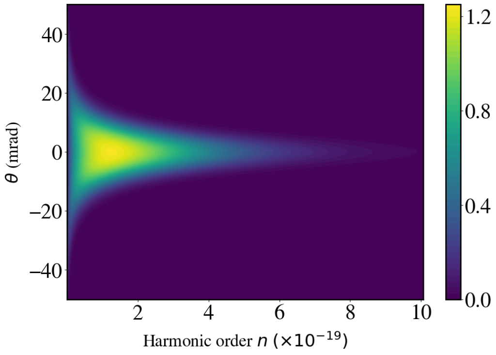
2D map of the power distribution
See Fig. 4.16.
|
1 2 3 4 5 6 7 8 9 10 11 12 13 14 15 16 17 18 19 20 21 22 23 24 25 26 27 28 29 30 31 32 33 34 35 36 37 38 39 40 41 42 43 44 45 46 47 |
e = 1.602e-19 #C c = 3.0e8 #m/s rho = 10 #m epsilon_0 = 8.854e-12 #F/m P_0 = (1.0/(8*np.pi**2*epsilon_0)) * (c*e**2 /(rho**2)) nsteps = 350 nmax = 10100000 thsteps = 100 n = np.arange(100,int((nmax-100)/nsteps)*nsteps, int(nmax/nsteps)) theta = np.linspace(-0.05,0.05, thsteps) gamma = 100 beta = np.sqrt(1-1/gamma**2)#beta = 0.999 power = np.zeros((nsteps, thsteps)) for i,j in enumerate(n): for k, th in enumerate(theta): power[i,k] = P_0*j**2 *beta**4 *( \ special.jvp(j,j*beta*np.cos(th))**2 + \ np.tan(th)**2 * special.jv(j,j*beta*np.cos(th))**2 / beta**2 ) x, y = np.meshgrid(n, 1000*theta) ls = LightSource(180, 45) with plt.style.context(('default')): plt.rcParams.update(synchrotron_style) fig, ax = plt.subplots(figsize=(12,8)) ctr = ax.contourf(x, y, power.T, 60, cmap=cm.viridis) plt.xticks(fontsize = 32) plt.yticks(fontsize = 32) plt.xlabel('Harmonic order $n$ $(\\times 10^{-19})$', fontsize=26, labelpad=10) plt.ylabel('$\\theta$ (mrad)', fontsize=26, labelpad=10) plt.xticks(ticks = [2e6, 4e6, 6e6, 8e6, 10e6],labels=("2", "4", "6", "8", "10"), fontsize = 32) cbar = plt.colorbar(ctr) cbar.set_ticks(ticks = [0, 0.4e-19, 0.8e-19, 1.2e-19],labels=("0.0", "0.4", "0.8", "1.2")) cbar.ax.tick_params(labelsize=32) plt.show() |
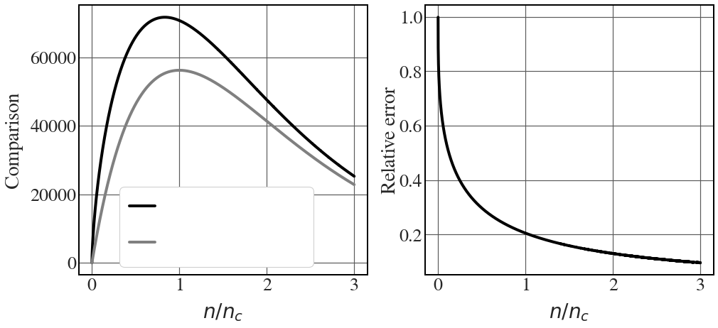
Asymptotic expansion of J_n^{'}(n \beta)
See Fig. 4.17. Note: the labels are added separately in the published book version.
|
1 2 3 4 5 6 7 8 9 10 11 12 13 14 15 16 17 18 19 20 21 22 23 24 25 26 27 28 29 30 31 |
gamma = 800.0 beta = np.sqrt(1.0 - 1.0/gamma**2) nsteps = 5000 nc = 1.5*gamma**3 nmax = int(3*nc) n = np.arange(1,int((nmax-100)/nsteps)*nsteps, int(nmax/nsteps)) original_function = n**2 * special.jvp(n,n*beta)**2 asymptotic_expansion = (n/(2*np.pi*gamma)) * np.exp(-2*n/(3*gamma**3)) with plt.style.context(('seaborn-v0_8-whitegrid')): plt.rcParams.update(synchrotron_style) fig, axs = plt.subplots(1, 2,figsize=(16,7)) fig.subplots_adjust(hspace=0) # Note: the labels are added separately in the published book version axs[0].plot(n/nc, original_function, 'k', lw = 4, label=" ") axs[0].plot(n/nc, asymptotic_expansion, 'gray', lw = 4, label=" ") axs[0].set_ylabel('Comparison', fontsize=28, labelpad=10) axs[0].tick_params(axis='y', labelsize=26) axs[0].tick_params(axis='x', labelsize=26) axs[0].set_xlabel('$n/n_{c}$', fontsize=28, labelpad=10) axs[1].plot(n/nc, (original_function-asymptotic_expansion)/original_function, 'k', lw = 4) axs[1].set_xlabel('$n/n_{c}$', fontsize=28, labelpad=10) axs[1].set_ylabel('Relative error', fontsize=28, labelpad=0) axs[1].tick_params(axis='y', labelsize=26) axs[1].tick_params(axis='x', labelsize=26) axs[0].legend(fontsize = 36, frameon=True, framealpha = 1, labelspacing=0.5, handlelength = 1, loc=(0.14,0.03)) |
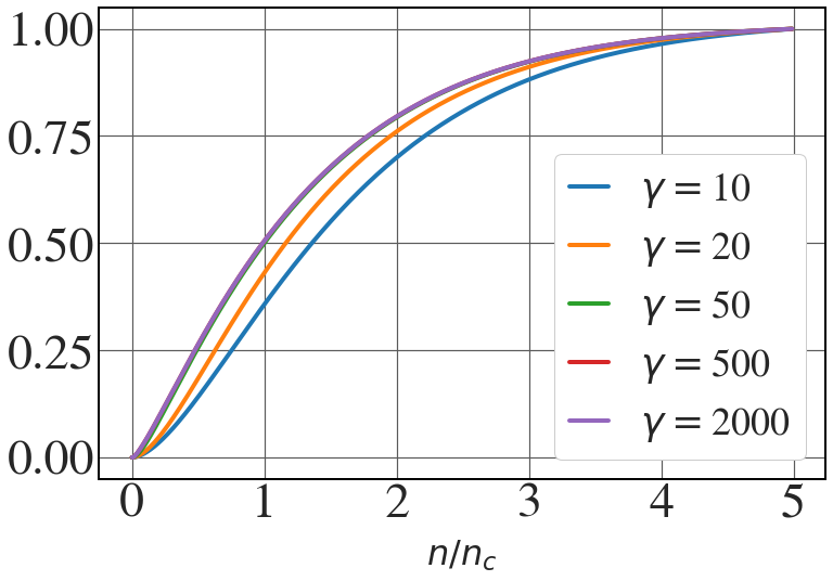
Numerical computation of critical harmonic number
See Fig. 4.18.
|
1 2 3 4 5 6 7 8 9 10 11 12 13 14 15 16 17 18 19 20 21 22 23 24 25 26 27 28 29 30 31 32 33 34 35 36 37 38 39 40 41 42 43 44 45 46 47 48 49 50 51 52 |
e = 1.602e-19 #C c = 3.0e8 #m/s rho = 10 #m epsilon_0 = 8.854e-12 #F/m P_0 = (1.0/(8*np.pi**2*epsilon_0)) * (c*e**2 /(rho**2)) nsteps = 500 nmax = 10000000 thsteps = 501 theta = np.linspace(-0.05,0.05, thsteps) dth = theta[1]-theta[0] with plt.style.context(('seaborn-whitegrid')): plt.rcParams.update(synchrotron_style) fig = plt.figure(figsize=(12,8)) for gamma in [10,20, 50, 500,2000]: nc = 1.5*gamma**3 n = np.arange(1,5*nc, int(5*nc/nsteps)) if n.shape[0]>nsteps: n = n[:nsteps] beta = np.sqrt(1-1/gamma**2)#beta = 0.999 power2d = np.zeros((nsteps, thsteps)) for i,j in enumerate(n): for k, th in enumerate(theta): power2d[i,k] = (27*gamma**2/(8*nc**2))*j**2 *( \ special.jvp(j,j*beta*np.cos(th))**2 + \ np.tan(th)**2 * special.jv(j,j*beta*np.cos(th))**2 / beta**2 )*np.cos(th) power1d = dth*np.sum(power2d, axis=1) cumul = np.zeros_like(n).astype('float32') for i,j in enumerate(n): cumul[i] = np.sum(power1d[:i])/np.sum(power1d) plt.plot(n/nc, cumul, lw = 4,label="$\\gamma=$"+str(gamma)) plt.yticks(ticks = [0, 0.25, 0.5, 0.75, 1], fontsize = 46) plt.xticks(fontsize = 46) plt.xlabel('$n/n_{c}$', fontsize=32, labelpad=10) plt.legend(fontsize = 36, frameon=True, loc='lower right', framealpha = 1, handlelength = 1) plt.show() |
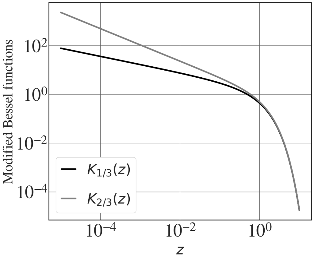
Modified Bessel functions of fractional order
See Fig. 4.19.
|
1 2 3 4 5 6 7 8 9 10 11 12 13 14 15 16 17 18 19 20 21 |
x = np.logspace(-5, 1, 10000) K13 = special.kv(1/3,x) K23 = special.kv(2/3,x) with plt.style.context(('seaborn-v0_8-whitegrid')): plt.rcParams.update(synchrotron_style) fig, axs = plt.subplots(1, 1, figsize=(12,10)) axs.loglog(x, K13, 'k', lw = 4, label="$K_{1/3}(z) $") axs.plot(x, K23, 'gray', lw = 4, label="$K_{2/3}(z)$") axs.set_ylabel('Modified Bessel functions', fontsize=36, labelpad=0) axs.set_xlabel('$z$', fontsize=36, labelpad=10) axs.legend(fontsize = 36, frameon=True, labelspacing=1.0, loc='lower left', framealpha = 1, handlelength = 1) axs.tick_params(axis='x', labelsize=46, pad=10) axs.tick_params(axis='y', labelsize=46) axs.yaxis.get_offset_text().set_fontsize(20) plt.show() |
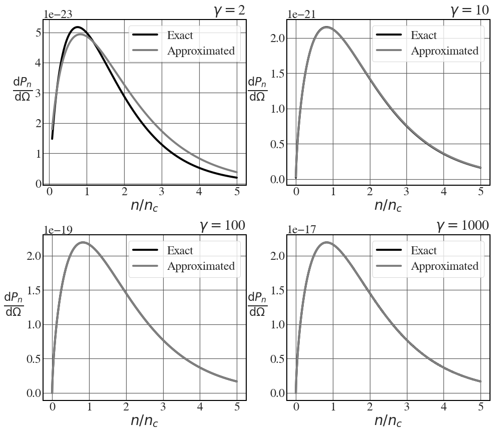
Comparison between exact and approximated spectrum
See Fig. 4.20.
|
1 2 3 4 5 6 7 8 9 10 11 12 13 14 15 16 17 18 19 20 21 22 23 24 25 26 27 28 29 30 31 32 33 34 35 36 37 38 39 40 41 |
e = 1.602e-19 #C c = 3.0e8 #m/s rho = 10 #m epsilon_0 = 8.854e-12 #F/m theta = 0.0000 nsteps = 5000 with plt.style.context(('seaborn-v0_8-whitegrid')): plt.rcParams.update(synchrotron_style) fig, axs = plt.subplots(2,2, figsize=(16,14)) fig.subplots_adjust(hspace=0.3) for ax, gamma in zip(axs.flat, [2,10,100,1000]): beta = np.sqrt(1.0-1.0/gamma**2) nc = 1.5*gamma**3 nmax = int(5.*nc) n = np.linspace(1, nmax, nsteps) P_tot = (1.0/(6*np.pi*epsilon_0)) * (c*e**2 /(rho**2)) * beta**4 * gamma**4 arg_j = (n*beta*np.cos(theta))#.astype('uint64') exact = P_tot*3*(n/nc)**2 * gamma**2 *(special.jvp(n,arg_j)**2 + np.tan(theta)**2 * \ special.jv(n,arg_j)**2 / beta**2 )/np.pi arg_k = 0.5*n/nc * (1+theta**2 * gamma**2)**1.5 approximated = P_tot*(1.0/np.pi**2)*(n/nc)**2 * \ ( (1+theta**2 * gamma**2)**2 *special.kv(2/3,arg_k)**2 /gamma**2 + \ theta**2 *(1+theta**2 * gamma**2)* special.kv(1/3,arg_k) )/np.pi ax.plot(n/nc, exact, 'k', lw = 4, label="Exact") ax.plot(n/nc, approximated, 'gray', lw = 4, label="Approximated") ax.set_ylabel('$\\frac{\mathrm{d}P_{n}}{\mathrm{d}\Omega}$', rotation=0, fontsize=32, labelpad=25) ax.set_xlabel('$n/n_{c}$', fontsize=28, labelpad=1) ax.legend(fontsize = 24, frameon=True, labelspacing=0.4, loc='upper right') ax.set_xticks([0,1,2,3,4,5], labels=['0','1','2','3','4','5']) ax.tick_params(axis='x', labelsize=24) ax.tick_params(axis='y', labelsize=24) ax.set_title('$\\gamma = $'+str(int(gamma)), fontsize=28, loc='right', pad=10) ax.yaxis.get_offset_text().set_fontsize(24) |
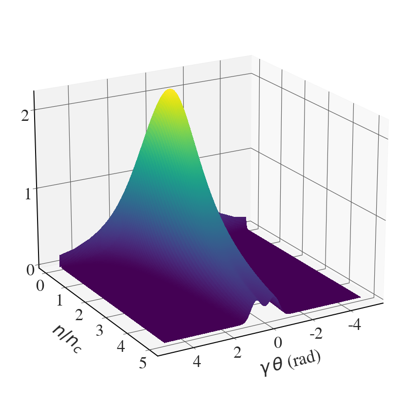
Surface plot of universal function
See Fig. 4.21.
|
1 2 3 4 5 6 7 8 9 10 11 12 13 14 15 16 17 18 19 20 21 22 23 24 25 26 27 28 29 30 31 32 33 34 35 36 37 38 39 40 41 42 43 44 45 46 47 48 49 50 51 |
e = 1.602e-19 #C c = 3.0e8 #m/s rho = 10 #m epsilon_0 = 8.854e-12 #F/m gamma = 1000 beta = np.sqrt(1.0-1.0/gamma**2) nc = int(1.5*gamma**3) nsteps = 350 nmax = int(5*nc) n = np.linspace(1, nmax, nsteps) thsteps = 200 theta = np.linspace(-0.005,0.005, thsteps) P_tot = (1.0/(6*np.pi*epsilon_0)) * (c*e**2 /(rho**2)) * beta**4 * gamma**4 power2d = np.zeros((nsteps, thsteps)) for i,j in enumerate(n): for k, th in enumerate(theta): argum = 0.5*j/nc * (1+th**2 * gamma**2)**1.5 power2d[i,k] = P_tot*(1.0/np.pi**2)*(j/nc)**2 * \ ( (1+th**2 * gamma**2)**2 *special.kv(2/3,argum)**2 /gamma**2 + \ th**2 *(1+th**2 * gamma**2)* special.kv(1/3,argum) )/np.pi X, Y = np.meshgrid(theta*gamma, n/nc) with plt.style.context(('seaborn-v0_8-whitegrid')): plt.rcParams.update(synchrotron_style) fig = plt.figure(figsize=(15,15)) ax1 = fig.add_subplot(111, projection='3d') surf1 = ax1.plot_surface(X, Y, power2d, rstride=1, cstride=1, cmap=cm.viridis, linewidth=0, antialiased=False) ax1.view_init(20, 60) z1 = np.around(np.max(power2d)/2, decimals=2) z2 = np.around(np.max(power2d), decimals=2) ax1.set_zticks([0,1e-17,2e-17]) ax1.set_zticklabels([0,1,2], fontsize=34) ax1.set_xticks([-4, -2, 0, 2, 4]) ax1.set_xticklabels([-4, -2, 0, 2, 4], fontsize=34) ax1.set_yticks([0, 1, 2, 3, 4, 5]) ax1.set_yticklabels([0, 1, 2, 3, 4, 5], fontsize=34) ax1.set_xlabel('$\\gamma \, \\theta$ (rad)', fontsize=36, labelpad=30) ax1.set_ylabel('$n/n_{c}$', fontsize=36, labelpad=30) plt.show() |
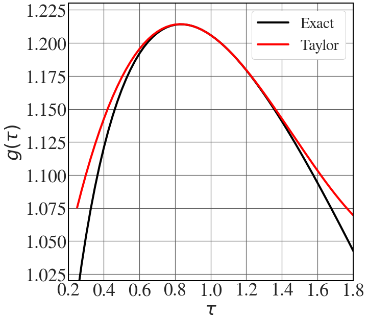
Taylor expansion of g(\tau)
Calculate Taylor expansion recursively and plot Fig. 4.22.
|
1 2 3 4 5 6 7 8 9 10 11 12 13 14 15 16 17 18 19 20 21 22 |
def cn_recursive(n): # Base case: c_0 = 0 if n == 0: return 0 # Recursive case: c_n = c_{n-1}/2 + 1/2^(n-1) else: return 0.5*cn_recursive(n-1) + 1/2**(n-1) def derivative_K(z, N): if N == 0: return z*special.kv(2/3,z/2) else: return cn_recursive(N)*special.kvp(2/3,z/2,n=N-1) + (z/2**N)*special.kvp(2/3,z/2,n=N) # Calculate the Taylor series up to fourth order ord = 4 a = np.zeros(ord) tayl_exp = np.zeros_like(x) for i in range(ord): test = derivative_K(x, i) a[i] = test[30]/np.math.factorial(i) tayl_exp += a[i]*(x-x[30])**i |
|
1 2 3 4 5 6 7 8 9 10 11 12 13 14 15 16 17 |
# Plot the Taylor expansion alongside the original function with plt.style.context(('seaborn-v0_8-whitegrid')): plt.rcParams.update(synchrotron_style) fig, ax = plt.subplots(figsize=(10,10)) ax.plot(x, x*special.kv(2/3,x/2), 'k', lw=4, label = "Exact") ax.plot(x, tayl_exp, 'r', lw=4, label="Taylor") ax.set_xlim([0.2, 1.8]) ax.set_ylim([1.02, 1.23]) plt.legend(fontsize = 30, frameon=True, framealpha=1) plt.xticks(fontsize = 36) plt.yticks(fontsize = 36) plt.xlabel('$\\tau$', fontsize=36) plt.ylabel("$g(\\tau)$", fontsize=36) |
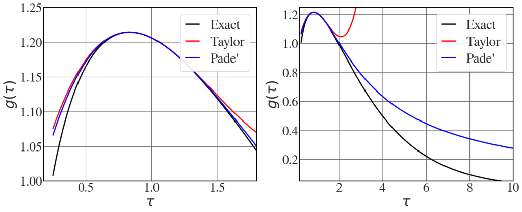
Padé approximant
The coefficients of the Padé approximant are derived from the Taylor series coefficients using the procedure described in the book by Baker (1975) that is cited on page 134. Note that the coefficients a[i] calculated in the previous section are needed for the calculations described in the computational exercise on page 111 and to plot Fig. 4.23.
|
1 2 3 4 5 6 7 8 9 10 11 12 13 14 15 16 17 18 19 20 21 22 23 24 25 26 27 28 29 30 31 32 33 34 |
A = a[0] D = (a[2]**2 - a[3]*a[1]) / (a[1]**2 -a[2]*a[0]) C = -a[0]*D/a[1] - a[2]/a[1] B = a[1]+a[0]*C pade = (A+B*(x-1)) / (1+C*(x-1)+D*(x-1)**2) with plt.style.context(('seaborn-v0_8-whitegrid')): plt.rcParams.update(synchrotron_style) fig, axs = plt.subplots(1,2, figsize=(21,8)) axs[0].plot(x, x*special.kv(2/3,x/2), 'k', lw=3,label = "Exact") axs[0].plot(x, tayl_exp, 'r', lw=3,label="Taylor") axs[0].plot(x, pade, 'b', lw=3,label="Pade'") axs[0].set_xlim([0.18, 1.8]) axs[0].set_ylim([1, 1.25]) axs[0].tick_params(axis='x', labelsize=32) axs[0].tick_params(axis='y', labelsize=32) axs[0].set_xlabel('$\\tau$', fontsize=36) axs[0].set_ylabel("$g(\\tau)$", fontsize=36) axs[0].legend(fontsize = 34, frameon=True, framealpha=0.9, loc = 'upper right', labelspacing=0.3, handlelength=1) axs[1].plot(x, x*special.kv(2/3,x/2), 'k', lw=3,label = "Exact") axs[1].plot(x, tayl_exp, 'r', lw=3,label="Taylor") axs[1].plot(x, pade, 'b', lw=3,label="Pade'") axs[1].set_xlim([0.18, 10]) axs[1].set_ylim([0.05, 1.25]) axs[1].tick_params(axis='x', labelsize=32) axs[1].tick_params(axis='y', labelsize=32) axs[1].set_xlabel('$\\tau$', fontsize=36) axs[1].set_ylabel("$g(\\tau)$", fontsize=36) axs[1].legend(fontsize = 34, frameon=True, framealpha=0.9, labelspacing=0.3, handlelength=1) plt.show() |
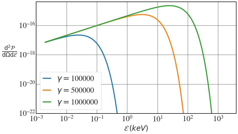
Synchrotron spectrum plotted as a function of energy
See Fig. 4.24.
|
1 2 3 4 5 6 7 8 9 10 11 12 13 14 15 16 17 18 19 20 21 22 23 24 25 26 27 28 29 30 31 32 33 34 35 36 37 38 39 40 |
e = 1.602e-19 #C c = 3.0e8 #m/s rho = 10 #m epsilon_0 = 8.854e-12 #F/m hbar = 6.582119569e-16 #eV s theta = 0.0000 nsteps = 25000 with plt.style.context(('seaborn-v0_8-whitegrid')): plt.rcParams.update(synchrotron_style) fig, ax = plt.subplots(1,1, figsize=(14,8)) for gamma in [1000,5000,10000]: beta = np.sqrt(1.0-1.0/gamma**2) omega_0 = beta*c/rho nc = 1.5*gamma**3 n = np.logspace(8, 14, nsteps) energy = hbar*omega_0*n/1000 # energy units in keV P_tot = (1.0/(6*np.pi*epsilon_0)) * (c*e**2 /(rho**2)) * beta**4 * gamma**4 arg_k = 0.5*n/nc * (1+theta**2 * gamma**2)**1.5 approximated = P_tot*(1.0/np.pi**2)*(n/nc)**2 * \ ( (1+theta**2 * gamma**2)**2 *special.kv(2/3,arg_k)**2 /gamma**2 + \ theta**2 *(1+theta**2 * gamma**2)* special.kv(1/3,arg_k) )/np.pi ax.loglog(energy, approximated, lw = 4, label="$\\gamma=$"+str(gamma)+"00") ax.set_ylabel('$\\frac{\mathrm{d}^{2} \\mathcal{P}}{\mathrm{d}\Omega\mathrm{d}\\mathcal{E}}$', rotation=0, fontsize=32, labelpad=35) ax.set_xlabel('$\\mathcal{E} \, (keV)$', fontsize=28, labelpad=5) ax.legend(fontsize = 30, frameon=True, labelspacing=0.5, loc='lower left', framealpha=1, handlelength=1) ax.tick_params(axis='x', labelsize=30, pad=10) ax.tick_params(axis='y', labelsize=30) ax.set_ylim(1e-22, 4e-15) ax.yaxis.get_offset_text().set_fontsize(20) plt.show() |
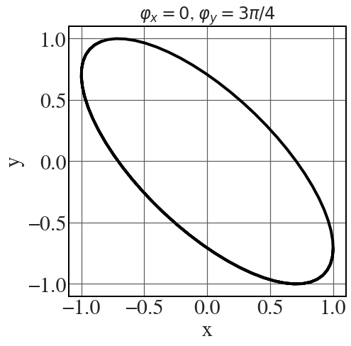
Polarisation: basic concepts
Plots of the polarisation ellipses in Fig. 4.27.
|
1 2 3 4 5 6 7 8 9 10 11 12 13 14 15 16 17 18 19 20 21 22 |
k_vec = 1 z = np.linspace(0,10,101) # Chnage phi_x and phi_y to generate the other cases phi_x = 0 phi_y = 3*np.pi/4# Ex_mod = 1 Ey_mod = 1 Ex = Ex_mod*np.cos(k_vec*z + phi_x) Ey = Ey_mod*np.cos(k_vec*z + phi_y) with plt.style.context(('seaborn-v0_8-whitegrid')): plt.rcParams.update(synchrotron_style) fig = plt.figure(figsize=(7,7)) plt.plot(Ex,Ey, 'k', lw = 4) plt.xticks(ticks = [-1,-0.5,0,0.5,1],fontsize = 30) plt.yticks(ticks = [-1,-0.5,0,0.5,1], fontsize = 30) plt.xlabel('x', fontsize=30) plt.ylabel("y", fontsize=30) plt.title("$\\varphi_{x} = 0$, $\\varphi_{y} = 3\pi/4$", fontsize=24) |
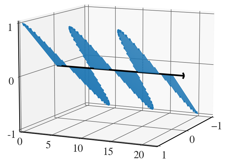
3D plots of polarisation components
See Fig. 4.28.
|
1 2 3 4 5 6 7 8 9 10 11 12 13 14 15 16 17 18 19 20 21 22 23 24 25 26 27 28 29 30 31 32 33 34 35 36 37 38 39 40 41 42 43 |
# These are the values for the components [phi_x, phi_y, Ex_mod, Ey_mod] to generate the different cases # Linear 0: [0,0,1,0] # Linear 45: [0,0,1,1] # Circular right: [0,-pi/2,1,1] # Circular left: [0,pi/2,1,1] k_vec = 2*np.pi/8 z = np.linspace(0,20,101) phi_x = 0 phi_y = 0 Ex_mod = 1 Ey_mod = 1 Ex = Ex_mod*np.cos(k_vec*z + phi_x) Ey = Ey_mod*np.cos(k_vec*z + phi_y) L = np.sqrt(Ex**2 + Ey**2) with plt.style.context(('seaborn-v0_8-whitegrid')): fig = plt.figure(figsize=(15,10)) plt.rcParams.update(synchrotron_style) ax = plt.subplot(projection='3d') ax.set_proj_type('persp') for i, j in enumerate(z): ax.quiver(0, j, 0, Ex[i], 0, Ey[i], linewidths=2, arrow_length_ratio=0.05) # Plot the axis ax.quiver(0,0,0, 0,22,0, arrow_length_ratio=0.01, linewidths=4, colors='black') ax.view_init(elev=10, azim=25) ax.set_ylim3d(0, 22) ax.set_xlim3d(-1, 1) ax.set_zlim3d(-1, 1) ax.set_zticks([-1,0,1]) ax.set_zticklabels([-1,0,1], fontsize=26) plt.xticks([-1, 0, 1], fontsize = 26) plt.yticks([0,5,10,15,20], fontsize = 26) plt.show() |
Polarisation ellipses of synchrotron radiation
See Fig. 4.30.
|
1 2 3 4 5 6 7 8 9 10 11 12 13 14 15 16 17 18 19 20 21 22 23 24 25 26 |
gamma = 1000 nc = int(1.5*gamma**3) phi = np.linspace(0,2*np.pi,360) beta = 1.0 - 0.5/gamma**2 with plt.style.context(('seaborn-v0_8-whitegrid')): plt.rcParams.update(synchrotron_style) fig, ax = plt.subplots(figsize=(10,10)) for th in [0, 0.00005, 0.0001, 0.0005]: E_par = np.cos(phi) E_perp = (np.tan(th)/beta)*special.jv(nc,nc*beta*np.cos(th))*np.sin(phi) / \ special.jvp(nc,nc*beta*np.cos(th)) ax.plot(E_par,E_perp, lw = 4, label = '$\\theta=$'+str(1000*th)+" mrad") plt.xticks(ticks = [-1,-0.5,0,0.5,1],fontsize = 36) plt.yticks(ticks = [-1,-0.5,0,0.5,1], fontsize = 36) plt.xlabel('Parallel', fontsize=36) plt.ylabel("Perpendicular", fontsize=36) plt.legend(fontsize = 30, frameon=True, ncol=2, loc='upper center', framealpha=1, handlelength = 1, handletextpad=0.5) plt.title("$\\gamma = 1000$", fontsize=30) plt.show() |

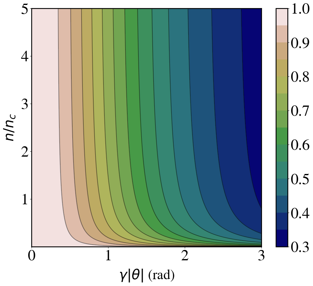
Eccentricity
See Fig. 4.31.
|
1 2 3 4 5 6 7 8 9 10 11 12 13 14 15 16 17 18 19 20 21 22 23 24 25 26 27 28 29 30 31 32 33 34 35 36 37 38 39 40 41 42 43 |
e = 1.602e-19 #C c = 3.0e8 #m/s rho = 10 #m epsilon_0 = 8.854e-12 #F/m gamma = 1000 beta = np.sqrt(1.0-1.0/gamma**2) nc = int(1.5*gamma**3) nsteps = 350 nmax = int(5*nc) n = np.linspace(1, nmax, nsteps) thsteps = 200 theta = np.linspace(0,0.003, thsteps) eccentricity = np.zeros((nsteps, thsteps)) for i,j in enumerate(n): for k, th in enumerate(theta): argum = 0.5*j/nc * (1+th**2 * gamma**2)**1.5 eccentricity[i,k] = np.sqrt( 1.0 - (th**2 * gamma**2 / (1+ th**2 * gamma**2))*\ (special.kv(1/3,argum)**2 /special.kv(2/3,argum)**2 ) ) X, Y = np.meshgrid(theta*gamma, n/nc) with plt.style.context(('default')): plt.rcParams.update(synchrotron_style) fig, ax = plt.subplots(figsize=(12,10)) ctr = ax.contourf(X, Y, eccentricity, 14, cmap=cm.gist_earth) ax.contour(X, Y, eccentricity, 14, colors='k', alpha=0.5) plt.xticks(fontsize = 36) plt.yticks(fontsize = 36) plt.ylabel('$n/n_{c}$', fontsize=32, labelpad=10) plt.xlabel('$\\gamma \\vert \\theta \\vert$ (rad)', fontsize=32, labelpad=10) cbar = plt.colorbar(ctr) cbar.ax.tick_params(labelsize=36) plt.show() |
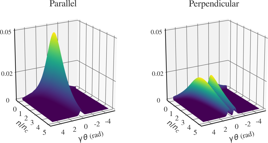
Spectral intensity associated with the two polarisation components
See Fig. 4.34. First calculate the two components.
|
1 2 3 4 5 6 7 8 9 10 11 12 13 14 15 16 17 18 19 20 21 22 23 |
epsilon_0 = 8.854e-12 #F/m rho = 10 #m gamma = 1000 beta = np.sqrt(1.0-1.0/gamma**2) nc = int(1.5*gamma**3) nsteps = 350 nmax = int(5*nc) thsteps = 200 n = np.arange(100,int((nmax-100)/nsteps)*nsteps, int(nmax/nsteps)) theta = np.linspace(-0.005,0.005, thsteps) parallel = np.zeros((nsteps, thsteps)) perpendicular = np.zeros((nsteps, thsteps)) P_tot = (1.0/(6*np.pi*epsilon_0)) * (c*e**2 /(rho**2)) * beta**4 * gamma**4 # Neglect the factor P_tot for i,j in enumerate(n): for k, th in enumerate(theta): argum = 0.5*j/nc * (1+th**2 * gamma**2)**1.5 parallel[i,k] = (1.0/np.pi**2)*(j/nc)**2 * (1+th**2 * gamma**2)**2 *special.kv(2/3,argum)**2/np.pi perpendicular[i,k] = (1.0/np.pi**2)*(j/nc)**2 * th**2 * gamma**2 * (1+th**2 * gamma**2)* \ special.kv(1/3,argum)/np.pi tot_power = parallel + perpendicular |
Then generate the plots.
|
1 2 3 4 5 6 7 8 9 10 11 12 13 14 15 16 17 18 19 20 21 22 23 24 25 26 27 28 29 30 31 32 33 34 35 36 37 38 39 40 41 42 43 44 45 46 47 48 49 |
X, Y = np.meshgrid(theta*gamma, n/nc) with plt.style.context(('seaborn-v0_8-whitegrid')): plt.rcParams.update(synchrotron_style) fig = plt.figure(figsize=(15,15)) ax1 = fig.add_subplot(121, projection='3d') ax2 = fig.add_subplot(122, projection='3d') surf1 = ax1.plot_surface(X, Y, parallel, rstride=1, cstride=1, cmap=cm.viridis, linewidth=0, antialiased=False) ax1.view_init(20, 60) z1 = np.around(np.max(tot_power)/2, decimals=2) z2 = np.around(np.max(tot_power), decimals=2) ax1.set_zticks([0,z1,z2]) ax1.set_zticklabels([0,z1,z2], fontsize=20) ax1.set_zlim3d(0,z2) ax1.zaxis.set_tick_params(pad=10) ax1.set_xticks([-4, -2, 0, 2, 4]) ax1.set_xticklabels([-4, -2, 0, 2, 4], fontsize=22) ax1.set_yticks([0, 1, 2, 3, 4, 5]) ax1.set_yticklabels([0, 1, 2, 3, 4, 5], fontsize=22) ax1.set_box_aspect((1, 1, 1.05)) ax1.set_xlabel('$\\gamma \, \\theta$ (rad)', fontsize=22, labelpad=15) ax1.set_ylabel('$n/n_{c}$', fontsize=22, labelpad=10) ax1.set_title('Parallel', fontsize=28) surf2 = ax2.plot_surface(X, Y, perpendicular, rstride=1, cstride=1, cmap=cm.viridis, linewidth=0, antialiased=False) ax2.view_init(20, 60) ax2.set_zticks([0,z1,z2]) ax2.set_zticklabels([0,z1,z2], fontsize=20) ax2.zaxis.set_tick_params(pad=10) ax2.set_zlim3d(0,z2) ax2.set_xticks([-4, -2, 0, 2, 4]) ax2.set_xticklabels([-4, -2, 0, 2, 4], fontsize=22) ax2.set_yticks([0, 1, 2, 3, 4, 5]) ax2.set_yticklabels([0, 1, 2, 3, 4, 5], fontsize=22) ax2.set_box_aspect((1, 1, 1.05)) ax2.set_xlabel('$\\gamma \, \\theta$ (rad)', fontsize=22, labelpad=15) ax2.set_ylabel('$n/n_{c}$', fontsize=22, labelpad=10) ax2.set_title('Perpendicular', fontsize=28) plt.savefig("polarisation_spectral_intensity.png", dpi=150) plt.show() |