Below is a set of python codes associated with Chapter 5 of Daniele Pelliccia and David M. Paganin, “Synchrotron Light: A Physics Journey from Laboratory to Cosmos” (Oxford University Press, 2025).
In order to run any of these python codes, you will need to include the following header file.
|
1 2 3 4 5 6 7 8 9 10 11 12 13 14 15 16 17 |
import numpy as np import matplotlib.pyplot as plt from mpl_toolkits.mplot3d import Axes3D from matplotlib import cm from matplotlib.colors import LightSource import matplotlib.gridspec as gridspec from scipy import special from sys import stdout synchrotron_style = { 'font.family': 'FreeSerif', 'font.size': 30, 'axes.linewidth': 2.0, 'axes.edgecolor': 'black', 'grid.color': '#5b5b5b', 'grid.linewidth': 1.2, } |
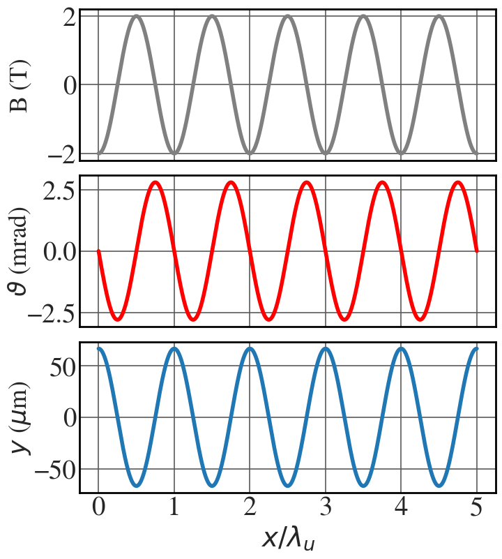
Electron trajectory
See Fig. 5.4.
|
1 2 3 4 5 6 7 8 9 10 11 12 13 14 15 16 17 18 19 20 21 22 23 24 25 26 27 28 29 30 31 32 33 34 35 36 37 38 |
# Constants B0 = 2 # T (tesla) l_u = 0.15 # m me = 9.11e-31 # kg el_energy = 3 # GeV c = 2.99792458e8 # m/s, speed of light gamma = 1000*el_energy/0.511 gamma = 10000 beta = 1.0 - 0.5/gamma**2 e_charge = 1.602e-19 # Define longitudinal coordinate x = np.linspace(0, 5*l_u, 1000) # Magnetic field amplitude B = -B0*np.cos(2*np.pi*x/l_u) # Deflection parameter K = e_charge*B0*l_u / (2 * np.pi * me * beta * c) deflection = -K*np.sin(2*np.pi*x/l_u)/gamma trajectory = K*l_u/(2*np.pi*gamma)* np.cos(2*np.pi*x/l_u) with plt.style.context(('seaborn-whitegrid')): plt.rcParams.update(synchrotron_style) fig, axs = plt.subplots(3, 1,figsize=(7.7,9), sharex=True) fig.subplots_adjust(hspace=0.1) axs[0].plot(x/l_u, B, 'grey', lw = 4) axs[0].tick_params(axis='y', labelsize=28) axs[0].set_ylabel('B (T)', fontsize=26, labelpad = 15) axs[1].plot(x/l_u, 1000*deflection, 'red', lw = 4) axs[1].tick_params(axis='y', labelsize=28) axs[1].set_ylabel('$\\vartheta$ (mrad)', fontsize=26, labelpad = -6) axs[2].plot(x/l_u, 1000000*trajectory, lw = 4) axs[2].tick_params(axis='y', labelsize=28) axs[2].set_xlabel('$x/\\lambda_u$', fontsize=28) axs[2].tick_params(axis='x', labelsize=28) axs[2].set_ylabel('$y$ ($\\mu$m)', fontsize=26, labelpad = 1) plt.show() |
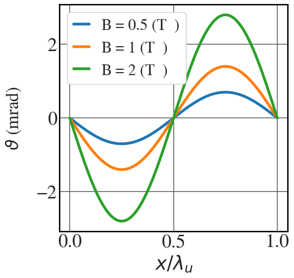
Plots of the deflection angle
These plots are obtained using the magnetic field as a parameter, as in Fig. 5.5(a).
|
1 2 3 4 5 6 7 8 9 10 11 12 13 14 15 16 17 18 19 20 21 22 |
gamma=10000 beta = 1.0 - 0.5/gamma**2 me = 9.11e-31 # kg e_charge = 1.602e-19 # C c = 2.99792458e8 # m/s, speed of light l_u = 0.15 # m # Define longitudinal coordinate x = np.linspace(0, l_u, 1000) with plt.style.context(('seaborn-whitegrid')): plt.rcParams.update(synchrotron_style) fig, ax = plt.subplots(1, 1,figsize=(6,6)) for magnetic_field in [0.5,1,2]: K = e_charge*magnetic_field*l_u / (2 * np.pi * me * beta * c) deflection = -K*np.sin(2*np.pi*x/l_u)/gamma ax.plot(x/l_u, 1000*deflection, lw = 4, label="B = "+str(magnetic_field)+" (T )") ax.tick_params(axis='y', labelsize=28) ax.set_ylabel('$\\vartheta$ (mrad)', fontsize=26, labelpad = 20) ax.set_xlabel('$x/\\lambda_u$', fontsize=28) ax.tick_params(axis='x', labelsize=28) plt.legend(fontsize=23, frameon=True, framealpha=1, handlelength=1) plt.show() |
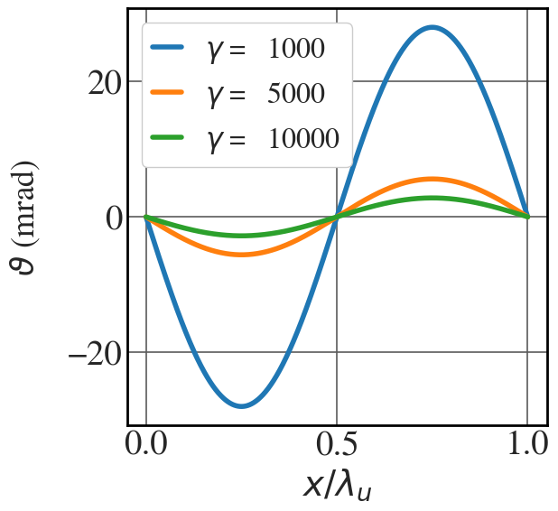
These plots are obtained using the Lorentz factor as a parameter, as in Fig. 5.5(b).
|
1 2 3 4 5 6 7 8 9 10 11 12 13 14 15 16 17 18 19 20 21 22 |
me = 9.11e-31 # kg e_charge = 1.602e-19 # C c = 2.99792458e8 # m/s, speed of light l_u = 0.15 # m B = 2 # T (tesla) # Define longitudinal coordinate x = np.linspace(0, l_u, 1000) with plt.style.context(('seaborn-whitegrid')): plt.rcParams.update(synchrotron_style) fig, ax = plt.subplots(1, 1,figsize=(6,6)) for gamma in [1000,5000,10000]: beta = 1.0 - 0.5/gamma**2 K = e_charge*B*l_u / (2 * np.pi * me * beta * c) deflection = -K*np.sin(2*np.pi*x/l_u)/gamma ax.plot(x/l_u, 1000*deflection, lw = 4, label="$\\gamma$ = "+str(gamma)) ax.tick_params(axis='y', labelsize=28) ax.set_ylabel('$\\vartheta$ (mrad)', fontsize=26, labelpad = 20) ax.set_xlabel('$x/\\lambda_u$', fontsize=28) ax.tick_params(axis='x', labelsize=28) plt.legend(fontsize=23, frameon=True, framealpha=1, handlelength=1) plt.show() |
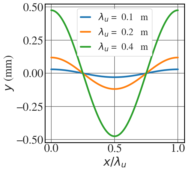
Plots of the electron trajectory
These plots are obtained using the wiggler period as a parameter, as in Fig. 5.5(c).
|
1 2 3 4 5 6 7 8 9 10 11 12 13 14 15 16 17 |
B0 = 2 # T (tesla) with plt.style.context(('seaborn-whitegrid')): plt.rcParams.update(synchrotron_style) fig, ax = plt.subplots(1, 1,figsize=(6,6)) for period in [0.1,0.2,0.4]: x = np.linspace(0, period, 1000) K = e_charge*B0*period / (2 * np.pi * me * beta * c) deflection = -K*np.sin(2*np.pi*x/period)/gamma trajectory = K*period*np.cos(2*np.pi*x/period) / (2*np.pi*gamma) ax.plot(x/period, 1000*trajectory, lw = 4, label="$\\lambda_u$ = "+str(period)+" m") ax.tick_params(axis='y', labelsize=28) ax.set_xlim(-0.05,1.05) ax.set_ylabel('$y$ (mm)', fontsize=28) ax.set_xlabel('$x/\\lambda_u$', fontsize=28) ax.tick_params(axis='x', labelsize=28) plt.legend(fontsize=23, frameon=True, framealpha=1, handlelength=1) plt.show() |
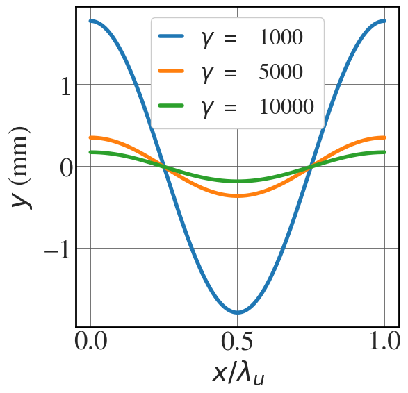
These plots are obtained using the Lorentz factor as a parameter, as in Fig. 5.5(d).
|
1 2 3 4 5 6 7 8 9 10 11 12 13 14 15 16 17 18 19 20 21 22 |
B0 = 2 # T (tesla) l_u = 0.15 x = np.linspace(0, l_u, 1000) with plt.style.context(('seaborn-whitegrid')): plt.rcParams.update(synchrotron_style) fig, ax = plt.subplots(1, 1,figsize=(6,6)) for gamma in [1000,5000,10000]: beta = 1.0 - 0.5/gamma**2 K = e_charge*B0*l_u / (2 * np.pi * me * beta * c) deflection = -K*np.sin(2*np.pi*x/l_u)/gamma trajectory = K*period*np.cos(2*np.pi*x/l_u) / (2*np.pi*gamma) ax.plot(x/l_u, 1000*trajectory, lw = 4, label="$\\gamma$ = "+str(gamma)) ax.tick_params(axis='y', labelsize=28) #ax.set_ylabel('$\\vartheta$ (mrad)', fontsize=24, labelpad = 20) ax.set_ylabel('$y$ (mm)', fontsize=28,labelpad=10) ax.set_xlabel('$x/\\lambda_u$', fontsize=28) ax.tick_params(axis='x', labelsize=28) plt.legend(fontsize=23, frameon=True, framealpha=1, handlelength=1) plt.show() |
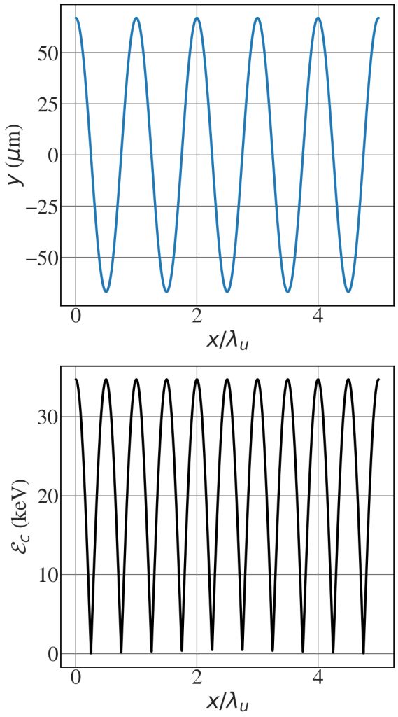
Electron trajectory and critical energy
See Fig. 5.7.
|
1 2 3 4 5 6 7 8 9 10 11 12 13 14 15 16 17 18 19 20 21 22 23 24 25 26 27 28 29 30 31 32 33 34 35 36 37 38 39 40 |
B0 = 2 # T (tesla) l_u = 0.15 # m me = 9.11e-31 # kg el_energy = 3 # GeV c = 2.99792458e8 # m/s, speed of light gamma = 10000 # 1000*el_energy/0.511 beta = 1.0 - 0.5/gamma**2 e_charge = 1.602e-19 hbar = 6.582119569e-16 # eV s so that the critical energy units is eV # Define longitudinal coordinate x = np.linspace(0, 5*l_u, 1000) # Magnetic field amplitude B = B0*np.cos(2*np.pi*x/l_u) # Deflection parameter K = e_charge*B0*l_u / (2 * np.pi * me * beta * c) deflection = -K*np.sin(2*np.pi*x/l_u)/gamma trajectory = K*l_u/(2*np.pi*gamma)* np.cos(2*np.pi*x/l_u) e_crit = (3*hbar*e_charge*np.abs(B)*gamma**2)/(2*me) with plt.style.context(('seaborn-whitegrid')): plt.rcParams.update(synchrotron_style) fig, ax = plt.subplots(2, 1,figsize=(10,20)) # fig.subplots_adjust(vspace=0.01) ax[0].plot(x/l_u, 1000000*trajectory, lw = 4)#, label="$\\gamma$ ="+str(gamma)) ax[0].tick_params(axis='y', labelsize=36) ax[0].set_ylabel('$y$ ($\\mu$m)', fontsize=36,labelpad=0) ax[0].set_xlabel('$x/\\lambda_u$', fontsize=36) ax[0].tick_params(axis='x', labelsize=36) ax[1].plot(x/l_u, e_crit/1000, 'black', lw = 4) ax[1].tick_params(axis='y', labelsize=36) ax[1].set_ylabel('$\\mathcal{E}_c$ (keV)', fontsize=36,labelpad=10) ax[1].set_xlabel('$x/\\lambda_u$', fontsize=36) ax[1].tick_params(axis='x', labelsize=36) plt.show() |
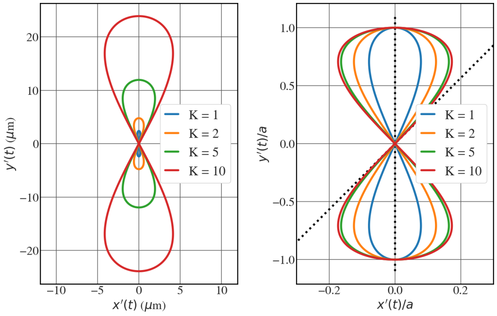
Electron trajectory: figure-eight
See Fig. 5.8.
|
1 2 3 4 5 6 7 8 9 10 11 12 13 14 15 16 17 18 19 20 21 22 23 24 25 26 27 28 29 30 31 32 33 34 35 36 37 38 39 40 41 42 43 44 45 46 47 48 49 50 51 52 53 54 55 56 |
l_u = 0.15 # m gamma = 10000 beta = 1 - 1/gamma**2 c = 2.99792458e8 # m/s, speed of light xt = np.linspace(-0.1,0.1,100) with plt.style.context(('seaborn-whitegrid')): plt.rcParams.update(synchrotron_style) #fig = plt.figure(figsize=(7,7)) fig, ax = plt.subplots(1, 2, figsize=(16,10)) fig.subplots_adjust(wspace=0.3) xx = np.linspace(-0.9, 0.9, 100) alpha_max = 1.0/(2*np.sqrt(2)*beta) ax[1].plot(alpha_max*xx,xx, 'k', ls = ':', lw = 4) ax[1].plot([0, 0], [-1.1, 1.1], 'k', ls = ':', lw = 4) for K in [1,2,5,10]: beta_bar = beta*(1-K**2/(4*gamma**2)) gamma_bar = 1.0/np.sqrt(1-beta_bar**2) om_u = beta*c t = np.linspace(0, 2*np.pi/om_u, 1000) y = K*l_u/(2*np.pi*beta*gamma)*np.sin(om_u*t) x = -K**2*l_u*gamma_bar/(16*np.pi*beta**2 *gamma**2)*np.sin(2*om_u*t) xred = 1e9*x/(K*gamma) yred = 1e9*y/(K*gamma) a = K*l_u/(2*np.pi*beta*gamma) ax[0].plot(1e6*x,1e6*y, lw = 4, label = "K = "+str(K)) ax[1].plot(x/a,y/a, lw = 4, label = "K = "+str(K)) ax[0].tick_params(axis='x', labelsize=24) ax[0].tick_params(axis='y', labelsize=24) ax[0].set_xlabel("$x'(t)$ ($\\mu$m)", fontsize=24) ax[0].set_ylabel("$y'(t)$ ($\\mu$m)", fontsize=24) ax[1].tick_params(axis='x', labelsize=24) ax[1].tick_params(axis='y', labelsize=24) ax[1].set_xlabel("$x'(t)/a$", fontsize=24) ax[1].set_ylabel("$y'(t)/a$", fontsize=24) ax[0].set_xlim([1000000*y.min()/2, 1000000*y.max()/2]) ax[1].set_xlim([-0.3, 0.3]) ax[0].legend(fontsize = 24, frameon=True, framealpha=1, handlelength=1) ax[1].legend(fontsize = 24, frameon=True, framealpha=1, handlelength=1) plt.show() |
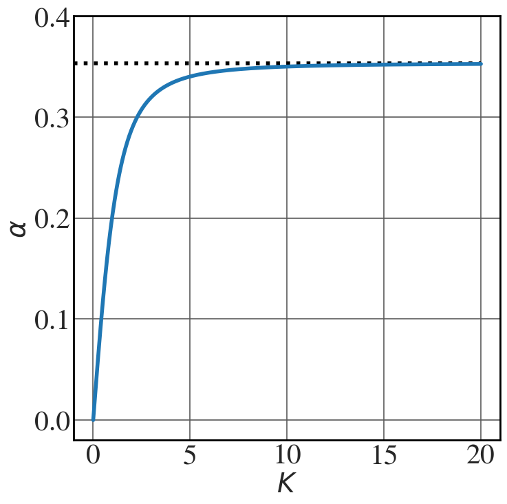
The opening angle of the figure-eight, shown in Fig. 5.9, can be plotted with the following code.
|
1 2 3 4 5 6 7 8 9 10 11 12 13 14 15 16 17 18 19 20 21 22 23 24 |
K=np.linspace(0,20,1000) with plt.style.context(('seaborn-whitegrid')): plt.rcParams.update(synchrotron_style) fig, ax = plt.subplots(1, 1,figsize=(8,8)) for gamma in [1000]: beta = 1.0 - 0.5/gamma**2 alpha = 0.25*K/np.sqrt(1+0.5*K**2) alpha_max = 1.0/(2*beta*np.sqrt(2)) ax.plot([-1,20], [alpha_max,alpha_max], 'k', lw=4, ls=':') ax.plot(K, alpha, lw = 4, label = "$\\gamma$ ="+str(gamma)) ax.set_xticks([0, 5,10,15,20]) #ax.plot(x/period, 1000*trajectory, lw = 4, label="$\\lambda_u$ ="+str(period)+" m") ax.tick_params(axis='y', labelsize=30) ax.set_ylim(-0.02,0.4) ax.set_xlim(-1,21) ax.set_ylabel('$\\alpha$', fontsize=28) ax.set_xlabel('$K$', fontsize=28) ax.tick_params(axis='x', labelsize=30) plt.show() |
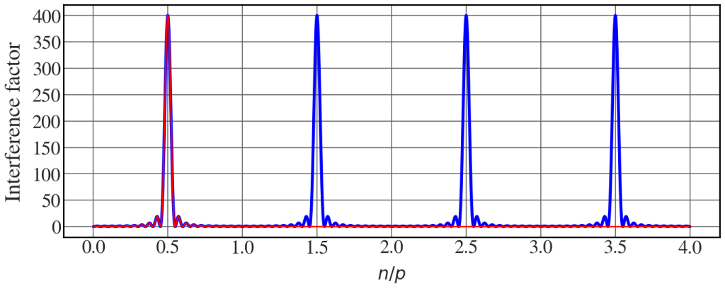
Interference factor \mathcal{I}
See Fig. 5.15.
|
1 2 3 4 5 6 7 8 9 10 11 12 13 14 15 16 17 18 19 20 21 22 23 24 25 26 27 28 29 30 31 32 |
e = 1.602e-19 # C c = 3.0e8 # m/s m_e = 9.109383702e-31 #kg, electron mass B0=10.0 # T (tesla) epsilon_0 = 8.854e-12 #F/m l_u = 0.15 #m N=10 gamma = 1000 beta = 1 - 1/gamma**2 rho_min = gamma*m_e*c/(e*B0) #m rho=10 omega_0 = c/rho theta=0.0 p = 2*np.pi*(2*rho)/l_u n = np.linspace(1,int(4*p),int(4*p)) f_n = l_u*n/(2*rho * gamma**2) interf_factor = (1-np.cos(2*np.pi*2*n*N/p))/(1+np.cos(2*np.pi*n/p)) interf_factor1 = 4*N**2*np.sin(N*2*np.pi*(n-1*p/2)/p)**2/(N*2*np.pi*(n-p/2)/p)**2 with plt.style.context(('seaborn-whitegrid')): plt.rcParams.update(synchrotron_style) fig, ax = plt.subplots(1,1, figsize=(16,5.7)) ax.plot(n/p, interf_factor, lw = 4, color='blue') ax.plot(n/p, interf_factor1, lw = 2, color='red') #ax.plot(n[:5000]/p, interf_factor2[:5000], lw = 2, color='red') plt.xlabel('$n/p$', fontsize=24, labelpad=10) plt.ylabel('Interference factor', fontsize=30, labelpad=10) plt.xticks(fontsize=26) plt.yticks(fontsize=26) plt.show() |
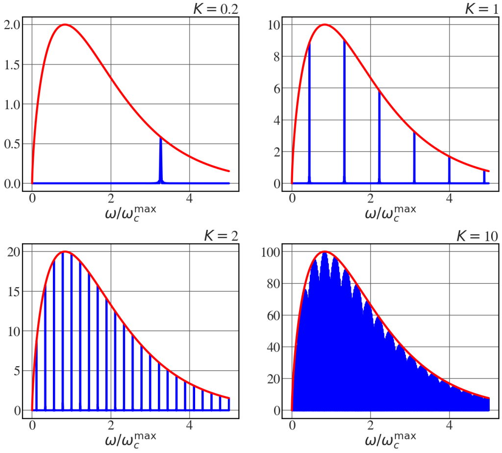
Transition between undulator and wiggler
See Fig. 5.16.
|
1 2 3 4 5 6 7 8 9 10 11 12 13 14 15 16 17 18 19 20 21 22 23 24 25 26 27 28 29 30 31 32 33 34 35 36 37 38 39 40 41 42 43 |
e = 1.602e-19 # C c = 3.0e8 # m/s m_e = 9.109383702e-31 # kg, electron mass B0=0.03#T epsilon_0 = 8.854e-12 # F/m N=100 gamma = 1000 beta = 1 - 1/gamma**2 l_u = 0.01 #m omega_u = 2*np.pi*c/l_u with plt.style.context(('seaborn-whitegrid')): plt.rcParams.update(synchrotron_style) fig, axs = plt.subplots(2,2, figsize=(16.5,14)) fig.subplots_adjust(hspace=0.3) for ax, K in zip(axs.flat, [0.2, 1, 2, 10]): rho_min = l_u*gamma/(2*np.pi*K) omega_c = 3 * gamma**2 * K * omega_u gammabar = gamma/np.sqrt(1+K**2/2) Mtot = 2000 omega = np.linspace(1,int(5*omega_c),100000) arg_k = omega/(2*omega_c) P_tot = e**2 * gamma**4 / (6*np.pi**2 * epsilon_0 *rho_min)*(3*omega/(4*np.pi*gamma*omega_c))**2 *\ special.kv(2/3,arg_k)**2 if K ==0.1: pmax = 4*N**2*np.max(P_tot) interference = np.zeros((P_tot.shape[0], Mtot)) for m in range(Mtot): interference[:,m] = np.sin(np.pi*N*(omega/(2*gammabar**2 * omega_u)-2*m-1))**2/(np.pi*N*(omega/(2*gammabar**2 * omega_u)-2*m-1))**2 int_factor = np.sum(interference, axis=1) P_id = 4*N**2* P_tot*int_factor # ax.plot(omega/omega_c, P_id/pmax, 'b', lw = 4) ax.plot(omega/omega_c, 4*N**2*P_tot/pmax, 'r', lw = 4) ax.set_xlabel('$\\omega/\omega_{c}^{\mathrm{max}}$', fontsize=28, labelpad=1) ax.tick_params(axis='x', labelsize=26) ax.tick_params(axis='y', labelsize=26) ax.set_title('$K = $'+str(K), fontsize=28, loc='right') ax.yaxis.get_offset_text().set_fontsize(20) plt.show() |
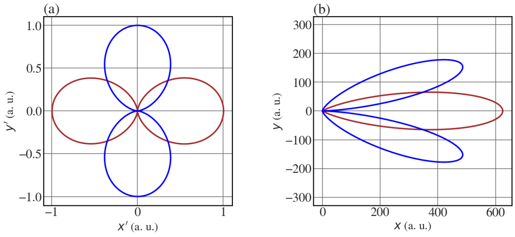
Relativistic effects in the undulator spectrum
Plot of the first two harmonics in different reference frames, as in Fig. 5.20.
|
1 2 3 4 5 6 7 8 9 10 11 12 13 14 15 16 17 18 19 20 21 22 23 24 25 26 27 28 29 30 31 32 33 34 35 36 37 38 39 40 41 42 43 44 45 46 47 48 |
theta = np.linspace(-np.pi, np.pi, 5000) K = 0.5 c = 3.0e8 #m/s l_u = 0.15 #m beta = [0.001, 0.8] with plt.style.context(('seaborn-whitegrid')): plt.rcParams.update(synchrotron_style) fig, axs = plt.subplots(nrows=1, ncols=2, figsize=(18.5, 7)) for i,j in enumerate(beta): gamma = 1/np.sqrt(1-j**2) print(gamma) beta_bar = j*(1-K**2/(4*gamma**2)) gamma_bar = 1.0/np.sqrt(1-beta_bar**2) om_u = j*c R1 = (1 - j*np.cos(theta))**(-4)*(1-np.sin(theta)**2/(gamma**2 * (1 - j*np.cos(theta))**2)) R2 = np.sin(theta)**2/(1 - j*np.cos(theta))**6 # Define parametric equations X1 = R1*np.cos(theta) #K*l_u/(2*np.pi*gamma)* Y1 = R1*np.sin(theta) X2 = R2*np.cos(theta) #K**2*j*l_u*gamma_bar/(16*np.pi*gamma**2)* Y2 = R2*np.sin(theta) axs[i].plot(X1, Y1, 'brown', lw = 3) axs[i].plot(X2, Y2, 'blue', lw = 3) if i==0: axs[i].set_ylim(-axs[i].get_xlim()[1], axs[i].get_xlim()[1]) axs[i].set_xlabel("$x'$ (a. u.)", fontsize=24) axs[i].set_ylabel("$y'$ (a. u.)", fontsize=24) axs[i].set_title(r"(a)", fontsize=30, loc='left') else: axs[i].set_ylim(-axs[i].get_xlim()[1]/2, axs[i].get_xlim()[1]/2) axs[i].set_xlabel("$x$ (a. u.)", fontsize=24) axs[i].set_ylabel("$y$ (a. u.)", fontsize=24) axs[i].set_title(r"(b)", fontsize=30, loc='left') axs[i].tick_params(axis='x', labelsize=26) axs[i].tick_params(axis='y', labelsize=26) axs[i].set_aspect('equal') plt.show() |
Numerical solution for the electron trajectory, as in Fig. 5.21.
|
1 2 3 4 5 6 7 8 9 10 11 12 13 14 15 16 17 18 19 20 21 22 23 24 25 26 27 28 29 30 31 32 33 34 35 36 37 38 39 40 41 42 43 44 45 46 47 48 49 50 51 52 53 54 55 56 57 58 59 60 61 62 63 64 65 66 67 68 69 70 71 72 73 74 75 76 77 |
def bisection(function, a, b, tolerance): c = (a+b)/2.0 Iters = 1 while np.abs(f(c)) >= tolerance: if f(a)*f(c) < 0: b = c else: a = c c = (a+b)/2 Iters += 1 return c c = 3.0e8 #m/s with plt.style.context(('seaborn-whitegrid')): plt.rcParams.update(synchrotron_style) fig = plt.figure(figsize=(15, 12), tight_layout=False) gs = gridspec.GridSpec(2, 2) ax1 = fig.add_subplot(gs[0, :]) ax12 = fig.add_subplot(gs[1, 0]) ax22 = fig.add_subplot(gs[1, 1]) for K in [0.1,1,10]: K_bar = K/np.sqrt(1+K**2/2) l_u = 0.15 #m omega_u = 2*np.pi*c/l_u k_u = 2*np.pi/l_u gamma = 1000 gamma_bar = gamma/np.sqrt(1+K**2/2) lp_u = l_u/gamma_bar kp_u = gamma_bar*k_u omegap_u = gamma_bar*omega_u tp = np.linspace(0, 10*lp_u/(2*c), 20000) xp = np.zeros_like(tp) for i, t in enumerate(tp): f = lambda x: x - K_bar**2/(8*kp_u)*np.sin(2*omegap_u*t+2*kp_u*x) a,b = -K_bar**2/(4*kp_u), K_bar**2/(4*kp_u) tol = 1e-11 xp[i] = bisection(f, a, b, tol) fx = np.abs(np.fft.fft(xp))**2 ax1.plot(tp[:2001]/lp_u/(2*c), xp[:2001] /(K_bar**2/(8*kp_u)), lw=3, label = "K = 00 "+str(K)) for i in range(2): if i ==0: ax12.plot(tp/(lp_u/(2*c)), xp /(K_bar**2/(8*kp_u)), lw=3) else: ax22.semilogy(np.arange(100)/10, fx[1:101] , label = "K = 00 "+str(K) , lw=3) ax1.set_xticks([0, tp[500]/lp_u/(2*c), tp[1000]/lp_u/(2*c), tp[1500]/lp_u/(2*c),tp[2000]/lp_u/(2*c)]) ax1.set_xticklabels(['0', '0.25','0.5','0.75', '1'], fontsize=24) ax1.set_yticks([-1, -0.5, 0, 0.5, 1]) ax1.set_yticklabels([-1, -0.5, 0, 0.5, 1], fontsize=24) ax1.set_xlabel("$2ct'/\\lambda'_u$", fontsize=28, labelpad=1) ax1.set_ylabel("$\\frac{8x'k'_{u}}{\\bar{K}^{2}}$", fontsize=38, rotation=0, labelpad=20) ax1.legend(fontsize=26, frameon=True, framealpha=1, handlelength=1) ax1.set_title(r"(a)", fontsize=26, loc='right') ax12.set_xticks([0, 2, 4, 6,8,10]) ax12.set_xticklabels(['0', '2', '4','6', '8', '10'], fontsize=24) ax12.set_xlabel("$2ct'/\\lambda'_u$", fontsize=28, labelpad=1) ax12.set_yticks([-1, -0.5, 0, 0.5, 1]) ax12.set_yticklabels([-1, -0.5, 0, 0.5, 1], fontsize=24) ax12.set_ylabel("$\\frac{8x'k'_{u}}{\\bar{K}^{2}}$", fontsize=38, rotation=0, labelpad=20) ax12.set_title(r"(b)", fontsize=26, loc='left') ax22.set_xticks([0, 1,2,3,4,5,6,7,8,9,10]) ax22.set_xticklabels([0, 2,4,6,8,10,12,14,16,18,20], fontsize=24) ax22.set_xlabel("$\\omega'/\\omega'_{u}$", fontsize=28, labelpad=1) ax22.set(yticklabels=[]) ax22.set_ylabel("Log power spectrum", fontsize=30, labelpad=1) ax22.set_title(r"(c)", fontsize=32, loc='right') plt.show() |

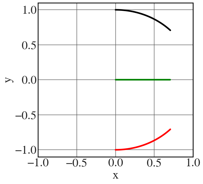
Polarisation ellipses
Portion of the polarisation ellipses for circularly polarised plane waves, as in Fig. 5.22.
|
1 2 3 4 5 6 7 8 9 10 11 12 13 14 15 16 17 18 19 20 21 22 23 24 25 26 27 28 29 30 31 |
omega = 1 t = np.linspace(0,np.pi/4,101) phi_x1 = np.pi/2 phi_y1 = 0 phi_x2 = np.pi/2 phi_y2 = np.pi Ex_mod = 1 Ey_mod = 1 Ex1 = Ex_mod*np.cos(phi_x1 - omega*t) Ey1 = Ey_mod*np.cos(phi_y1 - omega*t) Ex2 = Ex_mod*np.cos(phi_x2 - omega*t) Ey2 = Ey_mod*np.cos(phi_y2 - omega*t) with plt.style.context(('seaborn-whitegrid')): plt.rcParams.update(synchrotron_style) fig = plt.figure(figsize=(7,7)) plt.plot(Ex1,Ey1, 'k', lw = 4) plt.plot(Ex2,Ey2, 'r', lw = 4) plt.plot(0.5*(Ex1+Ex2),0.5*(Ey1+Ey2), 'g', lw = 4) plt.xticks(ticks = [-1,-0.5,0,0.5,1],fontsize = 30) plt.yticks(ticks = [-1,-0.5,0,0.5,1], fontsize = 30) plt.xlabel('x', fontsize=30) plt.ylabel("y", fontsize=30) plt.show() |
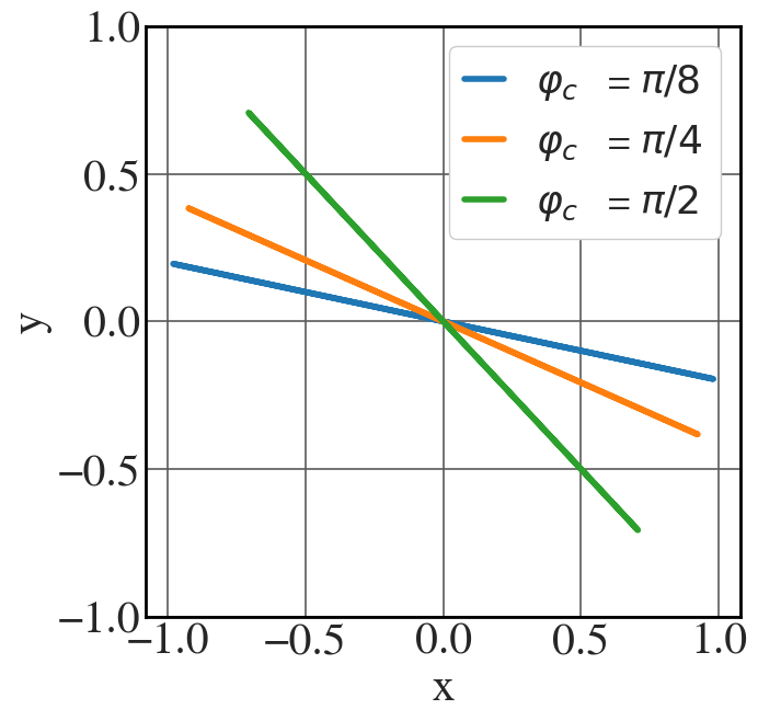
Polarisation ellipses corresponding to eqn (5.145), as in Fig. 5.23.
|
1 2 3 4 5 6 7 8 9 10 11 12 13 14 15 16 17 18 19 20 21 22 23 24 25 26 27 28 29 30 31 32 33 |
omega = 1 t = np.linspace(0,4*np.pi/2,101) phi_x1 = np.pi/2 phi_y1 = 0 phi_x2 = np.pi/2 phi_y2 = np.pi Ex_mod = 1 Ey_mod = 1 label_phase = ['$\\pi/8$', '$\\pi/4$', '$\\pi/2$'] with plt.style.context(('seaborn-whitegrid')): plt.rcParams.update(synchrotron_style) fig = plt.figure(figsize=(7,7)) for i, phi_c in enumerate([np.pi/8, np.pi/4, np.pi/2]): Ex1 = Ex_mod*np.cos(phi_x1 - omega*t) Ey1 = Ey_mod*np.cos(phi_y1 - omega*t) Ex2 = Ex_mod*np.cos(phi_x2 - omega*t + phi_c) Ey2 = Ey_mod*np.cos(phi_y2 - omega*t + phi_c) plt.plot(0.5*(Ex1+Ex2),0.5*(Ey1+Ey2), lw = 4, label = '$\\varphi_{c}$ = '+label_phase[i]+' ') plt.xticks(ticks = [-1,-0.5,0,0.5,1],fontsize = 30) plt.yticks(ticks = [-1,-0.5,0,0.5,1], fontsize = 30) plt.xlabel('x', fontsize=30) plt.ylabel("y", fontsize=30) plt.legend(fontsize=26, frameon = True, framealpha=1, handlelength=1) plt.show() |
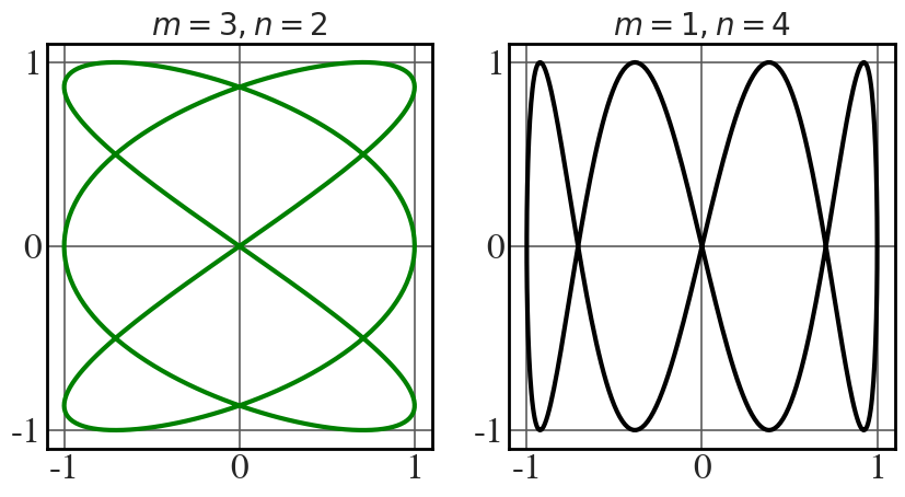
Lissajous figures
See Fig. 5.27.
|
1 2 3 4 5 6 7 8 9 10 11 12 13 14 15 16 17 18 19 20 |
x = np.linspace(0,2*np.pi, 360) with plt.style.context(('seaborn-whitegrid')): plt.rcParams.update(synchrotron_style) fig, axs = plt.subplots(nrows=1, ncols=2, figsize=(10, 4.8), tight_layout=False) axs[0].plot(np.sin(3*x), np.sin(2*x), 'g',lw=3) axs[0].set_xticks([-1,0, 1]) axs[0].set_yticks([-1,0, 1]) axs[0].set_xticklabels([-1,0, 1], fontsize=24) axs[0].set_yticklabels([-1,0, 1], fontsize=24) axs[0].set_title("$ m=3, n=2 $", fontsize=20) axs[1].plot(np.sin(1*x), np.sin(4*x), 'k',lw=3) axs[1].set_xticks([-1,0, 1]) axs[1].set_yticks([-1,0, 1]) axs[1].set_xticklabels([-1,0, 1], fontsize=24) axs[1].set_yticklabels([-1,0, 1], fontsize=24) axs[1].set_title("$ m=1, n=4 $", fontsize=20) plt.show() |