Below is a set of python codes associated with Chapter 11 of Daniele Pelliccia and David M. Paganin, “Synchrotron Light: A Physics Journey from Laboratory to Cosmos” (Oxford University Press, 2025).
In order to run any of these python codes, you will need to include the following header.
|
1 2 3 4 5 6 7 8 9 10 11 12 |
from scipy import special import numpy as np import matplotlib.pyplot as plt synchrotron_style = { 'font.family': 'FreeSerif', 'font.size': 30, 'axes.linewidth': 2.0, 'axes.edgecolor': 'black', 'grid.color': '#5b5b5b', 'grid.linewidth': 1.2, } |
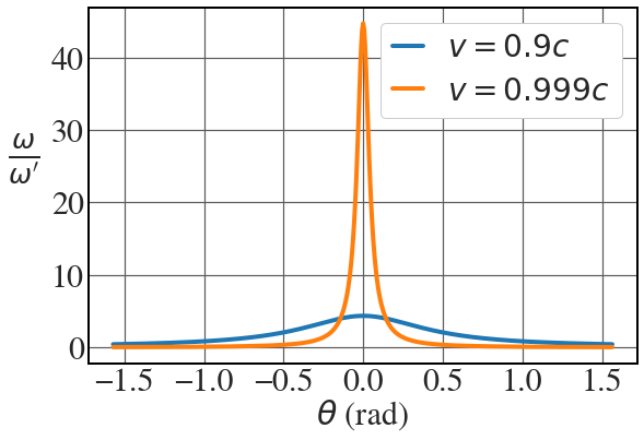
Doppler shift
See Fig. 11.2
|
1 2 3 4 5 6 7 8 9 10 11 12 13 14 15 16 17 18 19 20 21 22 |
c = 1. # set the speed of light in natural unit v1 = 0.9 v2 = 0.999 beta1 = v1/c beta2 = v2/c gamma1 = 1.0/ np.sqrt(1.0 - v1**2/c**2) gamma2 = 1.0/ np.sqrt(1.0 - v2**2/c**2) theta = np.linspace(-np.pi/2, np.pi/2, 500, endpoint=False) fig = plt.figure(figsize=(9,6)) with plt.style.context(('seaborn-v0_8-whitegrid')): plt.rcParams.update(synchrotron_style) plt.plot(theta,1.0/(gamma1*(1-beta1*np.cos(theta))), lw=4, label="$v = 0.9c$") plt.plot(theta,1.0/(gamma2*(1-beta2*np.cos(theta))), lw=4, label="$v = 0.999c$") plt.xlabel('$\\theta$ (rad)', fontsize=30, labelpad=0) plt.ylabel("$\\frac{\omega}{\omega'}$", rotation=0, fontsize=36, labelpad=25) plt.xticks(fontsize = 30) plt.yticks(fontsize = 30) plt.legend(fontsize = 28, frameon=True, handlelength=1, framealpha=1) |
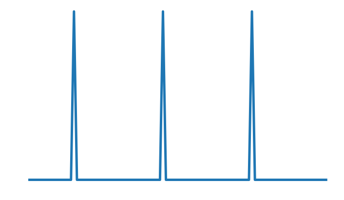
Dirac comb
This code snippet produces a basic version of the Dirac comb plotted in Fig. 11.3(b).
|
1 2 3 4 5 6 7 8 9 |
N, n = 101, 30 def f(i): return ((i-15) % n == 0) * 1 comb = np.fromfunction(f, (N,), dtype=int) plt.figure(figsize = (12,7)) plt.plot(comb, lw=5) plt.axis('off') plt.show() |
Spatial and temporal structure of synchrotron light
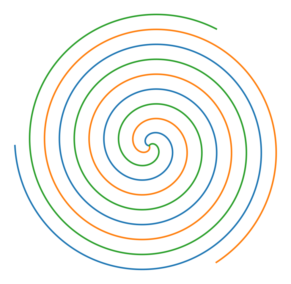
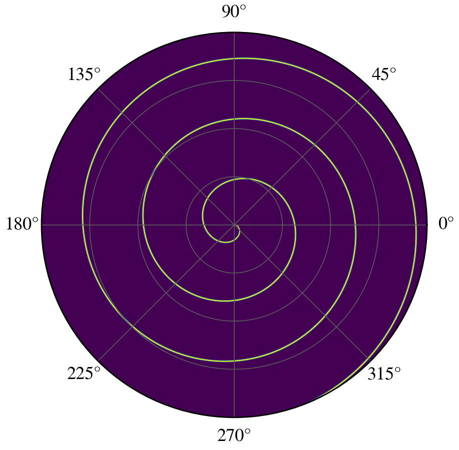
Archimedean spirals
See Fig. 11.11.
|
1 2 3 4 5 6 7 8 9 10 11 12 |
phi = np.linspace(0,6*np.pi, 10000) r = [phi, phi, phi ] offset = [0, 2*np.pi/3, 4*np.pi/3] plt.figure(figsize=[20,20]) for i,radius in enumerate(r): x = -radius*np.cos(phi-offset[i]) y = radius*np.sin(phi-offset[i]) plt.plot(x,y, lw=6) plt.axis("off") plt.show() |
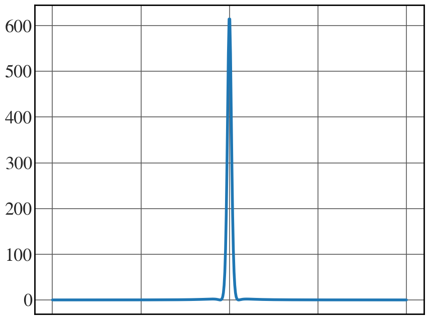
Auxiliary function f(s, \beta)
See Figs. 11.12(a) and 11.13(a).
|
1 2 3 4 5 6 7 8 9 10 11 12 13 14 15 16 17 |
bbeta = 0.8 # replace with 0.4 for Fig. 11.13(a) n = 1 s = np.linspace(-np.pi,np.pi, 500) aux = np.zeros_like(s) for n in np.arange(-100,100,1): aux = aux + n*np.exp(1j*n*s)*special.jvp(n, n*bbeta) auxil = np.abs(aux)**2 with plt.style.context(('seaborn-v0_8-whitegrid')): plt.rcParams.update(synchrotron_style) fig,ax = plt.subplots(figsize=(10,8)) plt.plot(s,auxil, lw=4) plt.xticks(fontsize = 24) plt.yticks(fontsize = 26) ax.set_xticks([-np.pi,-np.pi/2, 0,np.pi/2,np.pi],labels=["", "", "", "",""]) plt.show() |
Spatial structure of instantaneous energy density for a fixed instant of time
See Figs. 11.12(b) and 11.13(b).
|
1 2 3 4 5 6 7 8 9 10 11 12 13 14 15 16 17 18 19 20 21 22 23 24 25 26 27 28 29 30 31 |
import tqdm bbeta = 0.8 # replace with 0.4 to generate Fig. 11.13(b) phi = np.linspace(0, 2*np.pi, 3600) r = np.arange(0, 20, 0.002) rr, theta = np.meshgrid(r, phi) values = np.random.random((phi.size, r.size)) s = theta + rr aux = np.zeros_like(s) n_max = 200 for n in tqdm.tqdm(np.arange(-n_max,n_max,1)): aux = aux + n*np.exp(1j*n*s)*special.jvp(n, n*bbeta) auxil = np.abs(aux)**2 with plt.style.context(('default')): plt.rcParams.update(synchrotron_style) fig, ax = plt.subplots(subplot_kw=dict(projection='polar'), figsize=(10,10)) ax.contourf(theta, rr, auxil, levels=200) ax.set_rticks([0,5, 10,15,20]) ax.set_yticklabels([]) ax.tick_params(axis='y', labelsize=26) ax.tick_params(axis='x', labelsize=26) positions = [0, np.pi/4, np.pi/2, 3*np.pi/4, np.pi, 5*np.pi/4, 3*np.pi/2, 7*np.pi/4] for i,j in enumerate(ax.get_xticklabels()): j.set_position((positions[i],-0.05)) plt.show() |
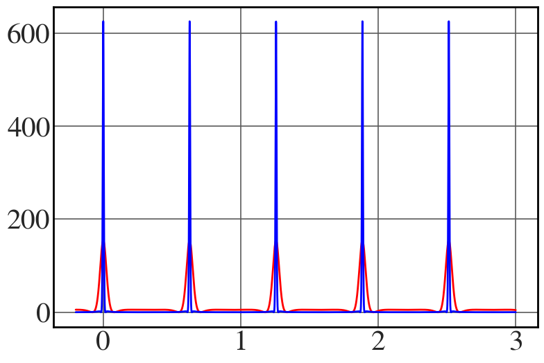
Temporal structure of synchrotron light
See Fig. 11.14.
|
1 2 3 4 5 6 7 8 9 10 11 12 13 14 15 16 17 18 19 20 21 22 23 24 |
bbeta1 = 0.8 bbeta2 = 0.4 n_max = 250 omega_0 = 10 t = np.linspace(-0.2,3, 10000) s = omega_0*t col = ['r', 'b'] with plt.style.context(('seaborn-v0_8-whitegrid')): plt.rcParams.update(synchrotron_style) fig = plt.figure(figsize=(9,6)) for i, bbeta in enumerate([0.4,0.8]): aux = np.zeros_like(s) for n in np.arange(-n_max,n_max,1): aux = aux + n*np.exp(1j*n*s)*special.jvp(n, n*bbeta) if bbeta == 0.4: auxil = 20*np.abs(aux)**2 else: auxil = np.abs(aux)**2 plt.plot(t,auxil, lw=2, color = col[i]) plt.show() |