Below is a set of python codes associated with Chapter 7 of Daniele Pelliccia and David M. Paganin, “Synchrotron Light: A Physics Journey from Laboratory to Cosmos” (Oxford University Press, 2025).
In order to run any of these python codes, you will need to include the following header file.
|
1 2 3 4 5 6 7 8 9 10 11 12 |
import numpy as np import matplotlib.pyplot as plt from scipy.special import genlaguerre, factorial synchrotron_style = { 'font.family': 'FreeSerif', 'font.size': 30, 'axes.linewidth': 2.0, 'axes.edgecolor': 'black', 'grid.color': '#5b5b5b', 'grid.linewidth': 1.2, } |
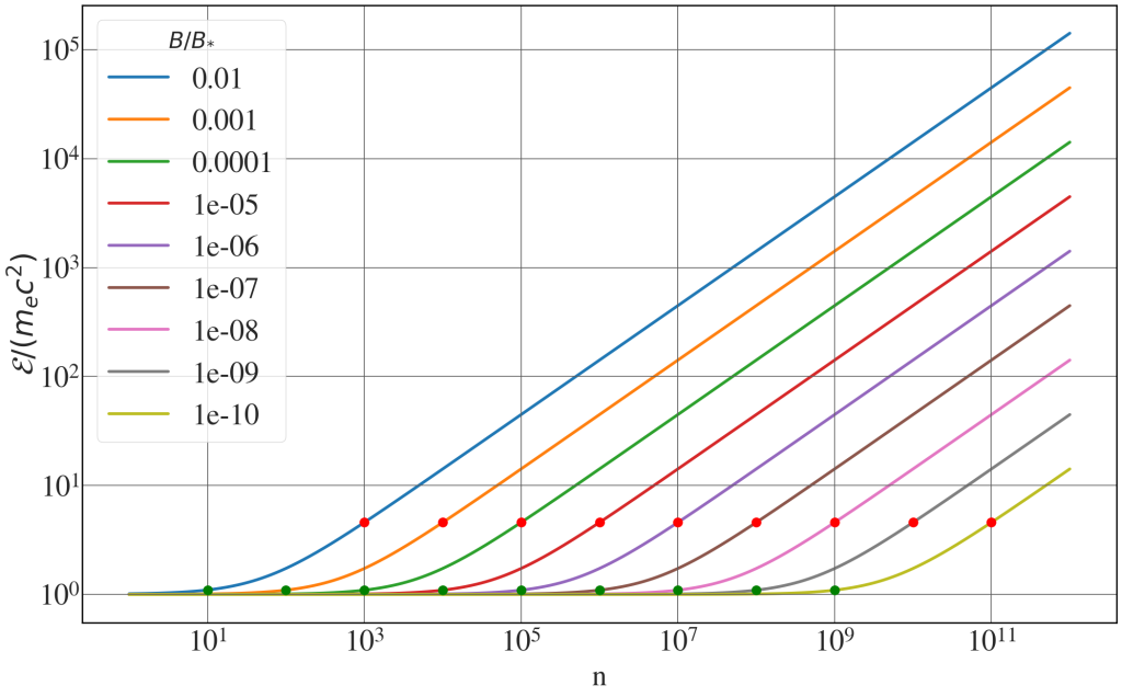
Allowed energy levels
See Fig. 7.2.
|
1 2 3 4 5 6 7 8 9 10 11 12 13 14 15 16 17 18 19 20 |
bb = np.logspace(-2,-10, 9) n = np.logspace(0,12,1000) with plt.style.context(('seaborn-v0_8-whitegrid')): plt.rcParams.update(synchrotron_style) fig, ax = plt.subplots(figsize=(25,15)) for ratio in bb: ax.scatter(0.1/ratio, np.sqrt(1+2*ratio*(0.1/ratio+0.5)), s = 150, c='g',zorder=10) ax.scatter(10/ratio, np.sqrt(1+2*ratio*(10/ratio+0.5)), s = 150, c='r',zorder=10) ax.loglog(n, np.sqrt(1+2*ratio*(n+0.5)), lw = 4, label = str(ratio), zorder=0) ax.tick_params(axis='x', labelsize=40, pad=10) plt.yticks(fontsize = 40) plt.xlabel('n', fontsize=40, labelpad=10) plt.ylabel("$\\mathcal{E}/ (m_{e}c^{2})$", rotation=90, fontsize=40, labelpad=-1) plt.legend(fontsize = 40, frameon=True, title="$B/B_{*}$") plt.show() |
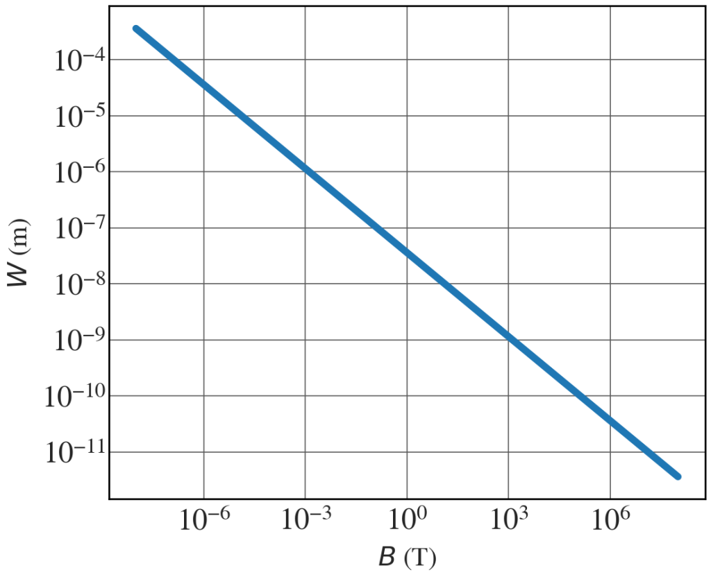
“Fuzzy ring” thickness
See Fig. 7.4.
|
1 2 3 4 5 6 7 8 9 10 11 12 13 14 15 16 17 18 19 |
bb = np.logspace(-8,8, 1000) hbar = 1.054571817e-34 ee = 1.602176634e-19 W = np.sqrt(2*hbar/(ee*bb)) with plt.style.context(('seaborn-v0_8-whitegrid')): plt.rcParams.update(synchrotron_style) fig, ax = plt.subplots(figsize=(12,10)) ax.loglog(bb, W, lw = 8) plt.xticks(fontsize = 34) plt.yticks(fontsize = 34) ax.tick_params(axis='x', pad=10) plt.xlabel('$B$ (T)', fontsize=30, labelpad=10) plt.ylabel('$W$ (m)', fontsize=30, labelpad=10) # plt.savefig('ring-thickness-versus-magnetic-field.png', dpi=600, transparent=False) plt.show() |
“Fuzzy ring” probability density
See Fig. 7.5.
|
1 2 3 4 5 6 7 8 9 10 11 12 13 |
r = np.linspace(0,20,5000) theta = np.linspace(0, 2*np.pi, 1000) bb=0.4 n=50 R, Th = np.meshgrid(r, theta) pkg = np.exp(-bb*R**2)*R**(2*n) X = R*np.cos(Th) Y = R*np.sin(Th) fig = plt.figure(figsize=(15,15)) plt.contourf(X,Y,pkg, levels=50, cmap='Purples') plt.axis('off') plt.show() |

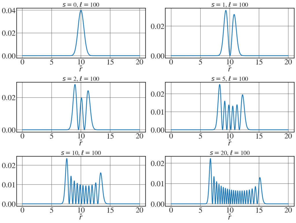
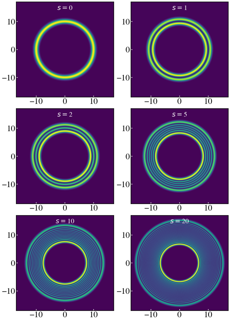
Radial line profiles of Klein-Gordon wavefunctions
See Fig. 7.6.
|
1 2 3 4 5 6 7 8 9 10 11 12 13 14 15 16 17 18 19 20 21 |
r = np.linspace(0,20,2000) ell = 100 with plt.style.context(('seaborn-v0_8-whitegrid')): plt.rcParams.update(synchrotron_style) fig, axs = plt.subplots(3,2, figsize=(16,12)) fig.subplots_adjust(wspace=5) for ax, s in zip(axs.flat, [0,1,2,5,10,20]): func = factorial(s)/(factorial(s+ell))*np.exp(-r**2)*r**(2*ell)*(genlaguerre(s, ell)(r**2))**2 ax.plot(r, func, lw=3) ax.set_title("$s= $"+str(s)+", $\\ell= $100", fontsize=24) ax.set_xlabel('$\\breve{r}$', fontsize=28, labelpad=1) ax.tick_params(axis='x', labelsize=30) ax.tick_params(axis='y', labelsize=30) plt.tight_layout() plt.show() |
Density plots of Klein-Gordon wavefunctions
See Fig. 7.7.
|
1 2 3 4 5 6 7 8 9 10 11 12 13 14 15 16 17 18 19 20 21 22 23 |
x = np.linspace(-17,17,1000) y = np.linspace(-17,17,1000) X,Y = np.meshgrid(x,y) ell = 100 with plt.style.context(('default')): plt.rcParams.update(synchrotron_style) fig, axs = plt.subplots(3,2, figsize=(11.5,16)) for ax, s in zip(axs.flat, [0,1,2,5,10,20]): func = factorial(s)/(factorial(s+ell))*np.exp(-X**2 - Y**2)*(X**2 + Y**2)**(ell)*(genlaguerre(s, ell)(X**2 + Y**2))**2 ax.contourf(X,Y,func, levels=50) ax.set_title("$s=$"+str(s), fontsize=24, loc='center', y=0.9, color='w') ax.set_xticks(ticks = [-10,0,10]) ax.tick_params(axis='x',direction='in', color='w', length=5, width=2) ax.set_yticks(ticks = [-10,0,10]) ax.tick_params(axis='y',direction='in', color='w', length=5, width=2) plt.tight_layout() plt.show() |
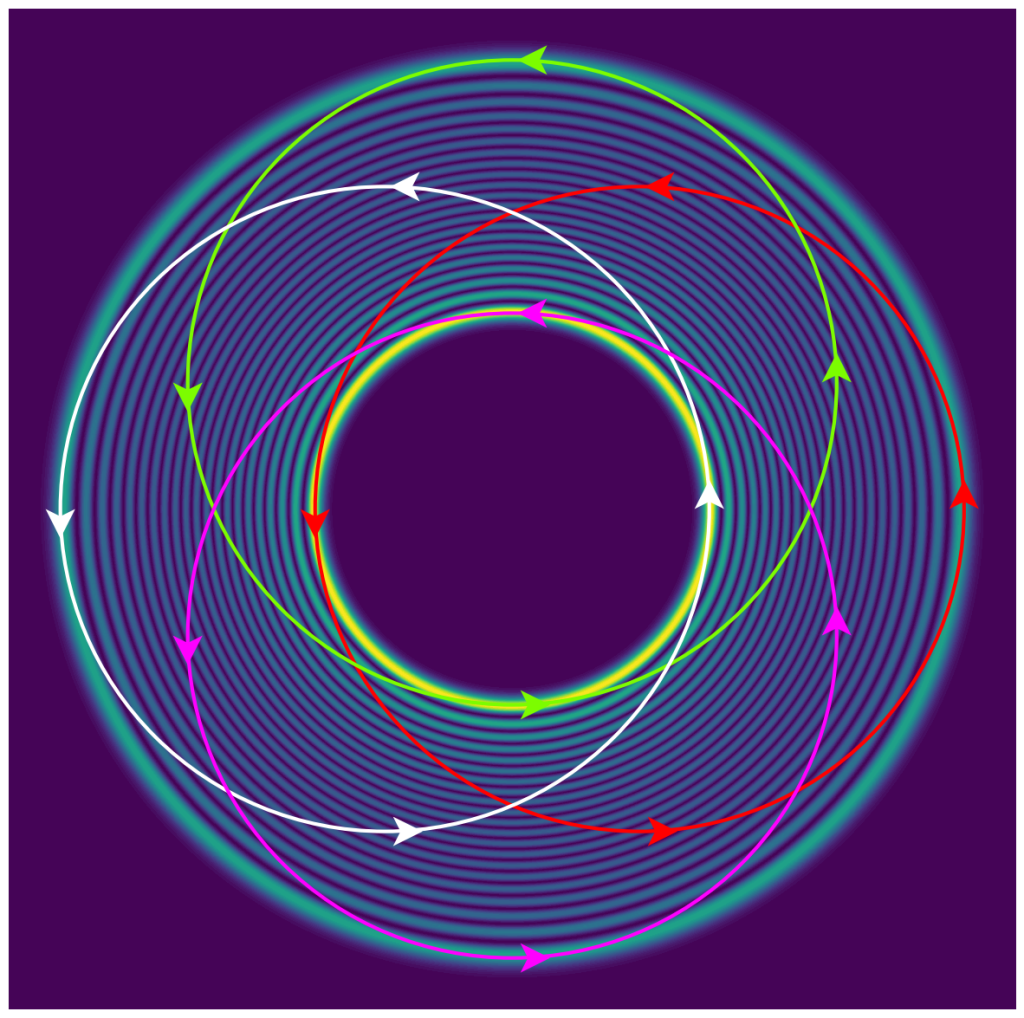
Klein-Gordon wavefunctions and classical orbits
See Fig. 7.10.
|
1 2 3 4 5 6 7 8 9 10 11 12 13 14 15 16 17 18 19 20 21 22 23 24 25 26 27 28 29 30 31 32 33 34 35 36 37 38 |
def plot_arrows(offsetx, offsety, color): plt.arrow(4.3+np.sqrt(ell+s)+offsetx,0+offsety, 0, 1, head_length=1,head_width=1, length_includes_head=True, \ linewidth=0, fc=color, overhang=0.25) plt.arrow(4.3-np.sqrt(ell+s)+offsetx,0+offsety, 0, -1, head_length=1,head_width=1, length_includes_head=True, \ linewidth=0, fc=color, overhang=0.25) plt.arrow(np.sqrt(ell+s)/2+offsetx,np.sqrt(ell+s)+offsety, -1, 0, head_length=1,head_width=1, length_includes_head=True, \ linewidth=0, fc=color, overhang=0.25) plt.arrow(np.sqrt(ell+s)/2+offsetx,-np.sqrt(ell+s)+offsety, 0.1, 0, head_length=1,head_width=1, length_includes_head=True, \ linewidth=0, fc=color, overhang=0.25) x = np.linspace(-17,17,1000) y = np.linspace(-17,17,1000) X,Y = np.meshgrid(x,y) ell = 100 s=20 circle1 = plt.Circle((4.3, 0), np.sqrt(s+ell), color=None, edgecolor='r', fill=False, lw=3) circle2 = plt.Circle((0, 4.3), np.sqrt(s+ell), color=None, edgecolor='lawngreen', fill=False, lw=3) circle3 = plt.Circle((-4.3, 0), np.sqrt(s+ell), color=None, edgecolor='white', fill=False, lw=3) circle4 = plt.Circle((0, -4.3), np.sqrt(s+ell), color=None, edgecolor='magenta', fill=False, lw=3) func = factorial(s)/(factorial(s+ell))*np.exp(-X**2 - Y**2)*(X**2 + Y**2)**(ell)\ *(genlaguerre(s, ell)(X**2 + Y**2))**2 fig, ax = plt.subplots(figsize=(15,15)) ax.contourf(X,Y,func, levels=50) ax.add_patch(circle1) ax.add_patch(circle2) ax.add_patch(circle3) ax.add_patch(circle4) plot_arrows(0,0,'r') plot_arrows(-4.3,4.3,'lawngreen') plot_arrows(-2*4.3,0,'white') plot_arrows(-4.3,-4.3,'magenta') plt.axis('off') plt.show() |
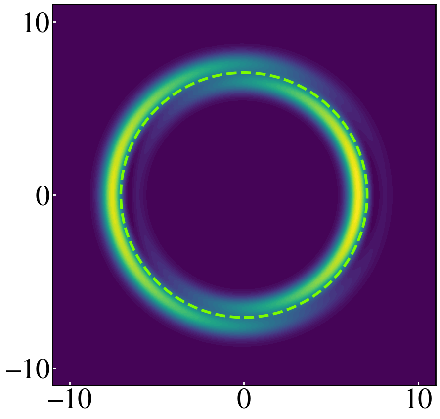
Linear combination of Klein-Gordon solutions
See Fig. 7.11.
|
1 2 3 4 5 6 7 8 9 10 11 12 13 14 15 16 17 18 19 20 21 22 23 24 25 26 27 28 29 30 31 32 33 34 35 |
x = np.linspace(-11,11,1000) y = np.linspace(-11,11,1000) X,Y = np.meshgrid(x,y) r = np.sqrt(X**2 + Y**2) phi = np.arctan2(Y,X) ell = 50 s=0 circle1 = plt.Circle((0, 0), np.sqrt(s+ell), color=None, edgecolor='lawngreen', fill=False, lw=4, ls='--') func1 = np.sqrt(factorial(s)/(factorial(s+ell)))*\ np.exp(1j*ell*phi)*\ np.exp(-0.5*r**2)*\ r**(ell)\ *(genlaguerre(s, ell)(r**2)) func2 = np.sqrt(factorial(s+1)/(factorial(s+ell)))*\ np.exp(1j*(ell-1)*phi)*\ np.exp(-0.5*r**2)*\ r**(ell-1)\ *(genlaguerre(s+1, ell-1)(r**2)) with plt.style.context(('default')): plt.rcParams.update(synchrotron_style) fig, ax = plt.subplots(figsize=(10,10)) ax.contourf(X,Y,np.abs(func1+func2)**2, levels=50) ax.add_patch(circle1) ax.set_xticks(ticks = [-10,0,10]) ax.tick_params(axis='x',direction='in', color='w', length=5, width=2, labelsize=42) ax.set_yticks(ticks = [-10,0,10]) ax.tick_params(axis='y',direction='in', color='w', length=5, width=2, labelsize=42) # plt.savefig("KleinGordonWavefunctions4.png", dpi=600) plt.show() |
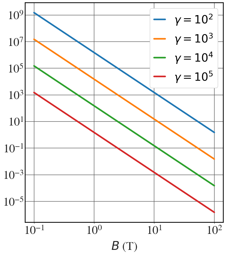
Spin-relaxation timescale
See Fig. 7.19.
|
1 2 3 4 5 6 7 8 9 10 11 12 13 14 15 16 17 18 19 20 21 22 23 |
hbar = 1.054571817e-34 # J*s m_e = 9.1093837015e-31 # kg c = 299792458 # m/s alpha = 1.0/137.035999084 Bstar = 4.41e9 # T (tesla) B = np.logspace(-1, 2, 1000) gs = ['$10^{2}$', '$10^{3}$', '$10^{4}$', '$10^{5}$'] with plt.style.context(('seaborn-v0_8-whitegrid')): plt.rcParams.update(synchrotron_style) fig, ax = plt.subplots(figsize=(9,10)) for i, gamma in enumerate([100,1000,10000,100000]): Tspinflip = (hbar/(m_e *c**2))*(Bstar/B)**3 * (gamma**(-2)/alpha) ax.loglog(B, Tspinflip, lw = 4, label = '$\\gamma=$'+gs[i]) plt.xticks(fontsize = 30) plt.yticks(fontsize = 30) ax.tick_params(axis='x', pad=5) plt.xlabel('$B$ (T)', fontsize=30, labelpad=10) plt.legend(fontsize=28, frameon=True, framealpha=1, handlelength=1) plt.show() |
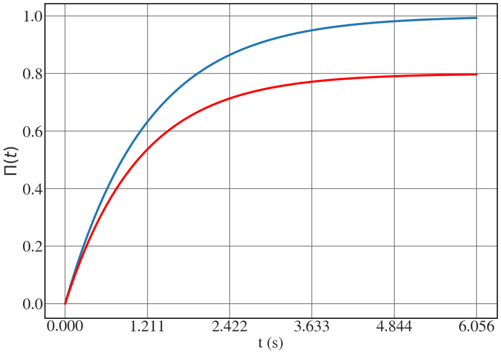
Degree of radiative polarisation
Gradual build-up of the degree of radiative polarisation, as in Fig. 7.20(a).
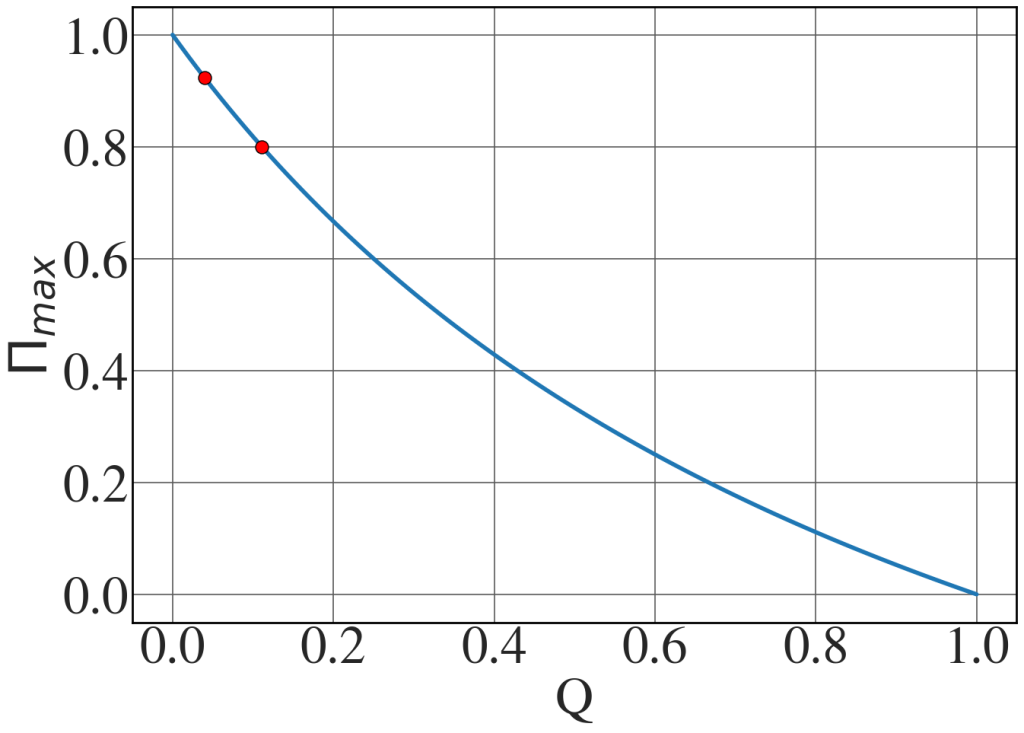
Maximum attainable spin polarisation, as in Fig. 7.20(b).
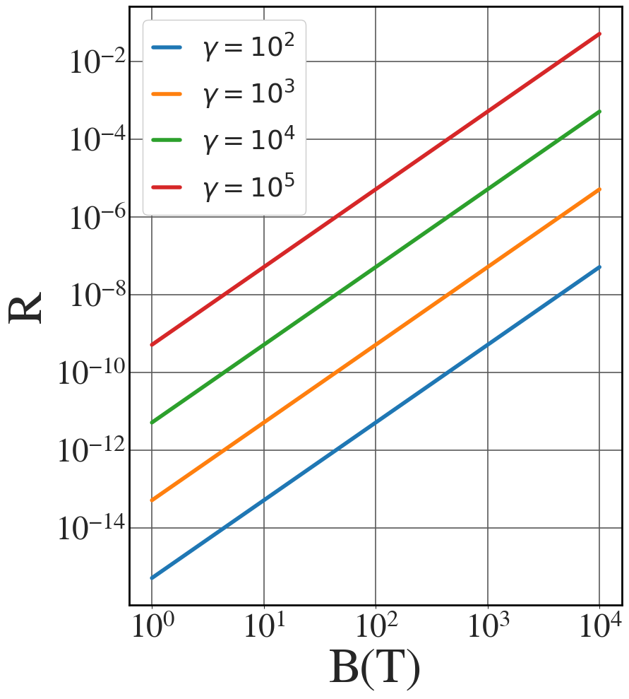
Ratio of spin-light versus synchrotron-radiation power
See Fig. 7.22.
|
1 2 3 4 5 6 7 8 9 10 11 12 13 14 15 16 17 18 19 20 21 |
hbar = 1.054571817e-34 # J*s ee = 1.602176634e-19 # C m_e = 9.1093837015e-31 # kg c = 299792458 #m/s B = np.logspace(0,4,500) # T (tesla) gg = ["$\\gamma = 10^{2}$", "$\\gamma = 10^{3}$", "$\\gamma = 10^{4}$", "$\\gamma = 10^{5}$"] with plt.style.context(('seaborn-v0_8-whitegrid')): plt.rcParams.update(synchrotron_style) fig, ax = plt.subplots(figsize=(9,11)) for i, gamma in enumerate(np.logspace(2,5,4)): R = (gamma*B*ee*hbar/(m_e**2 * c**2))**2 ax.loglog(B,R, lw = 4, label=gg[i]) plt.legend(fontsize=27, frameon=True, framealpha=1, handlelength=1) plt.xticks(fontsize = 34) plt.yticks(fontsize = 34) ax.tick_params(axis='x', pad=5) ax.set_xlabel("B(T)", fontsize=50) ax.set_ylabel("R", fontsize=50) plt.show() |
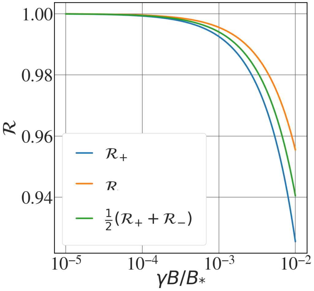
Quantum corrections to emitted synchrotron power
See Fig. 7.23.
|
1 2 3 4 5 6 7 8 9 10 11 12 13 14 15 16 17 18 19 20 21 22 23 |
x = np.logspace(-5,-2, 1000) Rplus = 1 - (1.5 + 55*np.sqrt(3)/16.0)*x Rminus = 1 - (-1.5 + 55*np.sqrt(3)/16.0)*x Ravg = 0.5*(Rplus+Rminus) with plt.style.context(('seaborn-v0_8-whitegrid')): plt.rcParams.update(synchrotron_style) fig, ax = plt.subplots(figsize=(12,12)) ax.semilogx(x,Rplus, lw = 4, label="$\\mathcal{R}_{+}$") ax.semilogx(x,Rminus, lw = 4, label="$\\mathcal{R}_{-}$") ax.semilogx(x,Ravg, lw = 4, label="$\\frac{1}{2} \\left( \\mathcal{R}_{+} + \\mathcal{R}_{-} \\right)$") plt.legend(fontsize=42 , frameon=True, framealpha=1, handlelength=1, labelspacing=1.0, borderpad=0.9) ax.set_yticks(ticks = [0.94,0.96,0.98, 1.0]) plt.xticks(fontsize = 48) plt.yticks(fontsize = 48) ax.tick_params(axis='x', pad=10) ax.set_ylabel('$\\mathcal{R}$', fontsize=50) ax.set_xlabel('$\\gamma B/B_{*}$', fontsize=50, labelpad=-10) plt.show() |
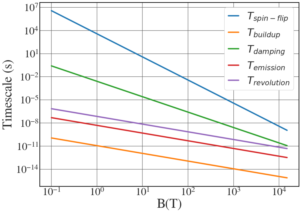
Characteristic timescales
See Fig. 7.25.
|
1 2 3 4 5 6 7 8 9 10 11 12 13 14 15 16 17 18 19 20 21 22 23 24 25 26 27 28 29 30 31 32 33 |
hbar = 1.054571817e-34 # J*s m_e = 9.1093837015e-31 # kg ee = 1.602176634e-19 # C eps_0 = 8.8541878128e-12 c = 299792458 # m/s alpha = 1.0/137.035999084 Bstar = 4.41e9 # T (tesla) gamma = 2000 B = np.linspace(0.1,15000,10000) Tspinflip = (hbar/(m_e *c**2))*(Bstar/B)**3 * (gamma**(-2)/alpha) Tbuildup = 2*m_e / (ee*B) Tdamping = (6*np.pi*eps_0 * m_e**3 * c**3) / (ee**4 * B**2 * gamma) Temission = (2 * np.pi * m_e) / (ee * alpha * B) Trevolution = (2 * np.pi * gamma * m_e) / (ee * B) with plt.style.context(('seaborn-v0_8-whitegrid')): plt.rcParams.update(synchrotron_style) fig, ax = plt.subplots(figsize=(14,10)) ax.loglog(B,Tspinflip, lw = 4, label="$T_{spin-flip}$") ax.loglog(B,Tbuildup, lw = 4, label="$T_{buildup}$") ax.loglog(B,Tdamping, lw = 4, label="$T_{damping}$") ax.loglog(B,Temission, lw = 4, label="$T_{emission}$") ax.loglog(B,Trevolution, lw = 4, label="$T_{revolution}$") plt.legend(fontsize=31, frameon=True, loc = 'upper right', framealpha=1, handlelength=1) plt.xticks(fontsize = 32) plt.yticks(fontsize = 32) ax.tick_params(axis='x', pad=5) ax.set_ylabel('Timescale (s)', fontsize=40) ax.set_xlabel('B(T)', fontsize=40) plt.show() |