Below is a set of python codes associated with Chapter 9 of Daniele Pelliccia and David M. Paganin, “Synchrotron Light: A Physics Journey from Laboratory to Cosmos” (Oxford University Press, 2025).
In order to run any of these python codes, you will need to include the following header.
|
1 2 3 4 5 6 7 8 9 10 11 12 13 14 15 16 17 18 19 20 21 |
import numpy as np import pandas as pd import matplotlib.pyplot as plt from matplotlib.colors import LogNorm from matplotlib.ticker import FormatStrFormatter from matplotlib import ticker import matplotlib as mpl from sys import stdout from mpl_toolkits.mplot3d import Axes3D from scipy import special from skimage import exposure from scipy import special synchrotron_style = { 'font.family': 'FreeSerif', 'font.size': 30, 'axes.linewidth': 2.0, 'axes.edgecolor': 'black', 'grid.color': '#5b5b5b', 'grid.linewidth': 1.2, } |
Spectrum of a single particle as a function of the pitch angle
See Fig. 9.6.
|
1 2 3 4 5 6 7 8 9 10 11 12 13 14 15 16 17 18 19 20 21 22 23 24 25 26 27 28 29 30 31 32 33 34 35 36 37 38 39 40 |
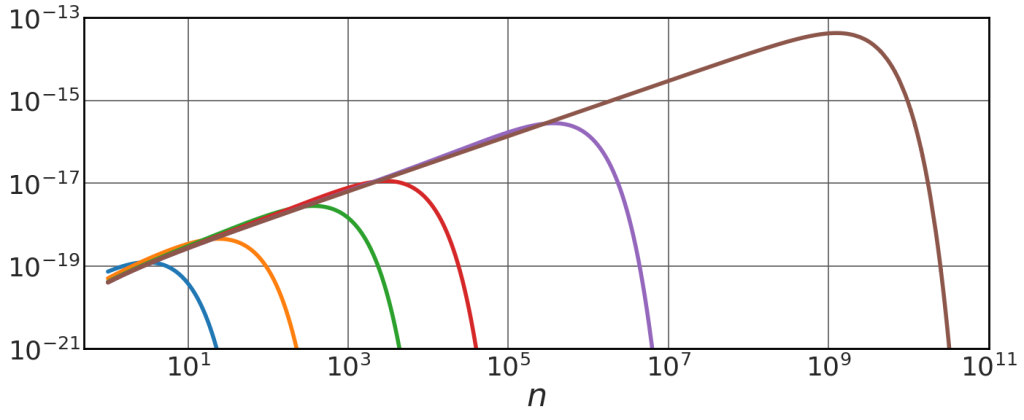
e = 1.602e-19 #C m = 9.10938356e-31 #kg c = 3.0e8 #m/s B = 10 #T epsilon_0 = 8.854e-12 #F/m gamma = 1000 nsteps = 50000 nc = 1.5*gamma**3 nmax = int(8*c) n = np.logspace(0, 11,nsteps) alpha_label = ["$0.5 \\times \\pi/2$","$0.75 \\times \\pi/2$","$0.9 \\times \\pi/2$", \ "$0.95 \\times \\pi/2$","$0.99 \\times \\pi/2$","$ \\pi/2$"] with plt.style.context(('seaborn-v0_8-whitegrid')): plt.rcParams.update(synchrotron_style) fig, ax= plt.subplots(figsize=(16,5.9)) for i, alpha in enumerate([np.pi/4, 0.75*np.pi/2,0.9*np.pi/2,0.95*np.pi/2,0.99*np.pi/2, np.pi/2]): theta = 0 beta_perp = np.sqrt(1.0-1.0/gamma**2)*np.sin(alpha) beta_par = np.sqrt(1.0-1.0/gamma**2)*np.cos(alpha) gamma_perp = 1.0/np.sqrt(1-beta_perp**2) v_perp = beta_perp*c # Argument of the Bessel functions arg_j = (n*beta_perp*np.cos(theta) / (1 - beta_par*np.sin(theta)) ) power_perp = ((e**4 * B**2 *n**2 * beta_perp**2)/(8*np.pi**2 * epsilon_0 * m**2 * c * gamma**2*(1-beta_par*np.sin(theta))**4 ))*\ (special.jvp(n,arg_j)**2 + ( (np.sin(theta) - beta_par) / (beta_perp*np.cos(theta)) )**2 *special.jv(n,arg_j)**2 / beta_perp**2 ) ax.loglog(n, power_perp, lw=4, label="$\\alpha =$"+alpha_label[i]) ax.set_ylim(1e-21,1e-13) ax.set_xlim(0.5,1e11) ax.tick_params(axis='x', labelsize=26, pad=5) ax.tick_params(axis='y', labelsize=26) ax.set_xlabel('$n$', fontsize=32, labelpad=1) plt.show() |
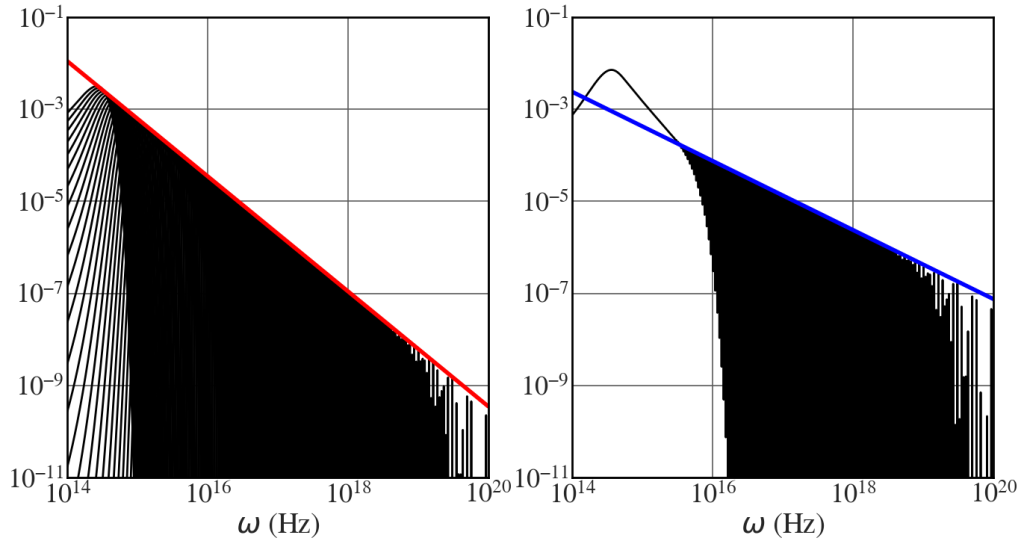
Effect of electron energy distribution on synchrotron-emission spectrum
Simulation of a collection of Gaussian spectral lines
See Fig. 9.8.
|
1 2 3 4 5 6 7 8 9 10 11 12 13 14 15 16 17 18 19 20 21 22 23 24 25 26 27 28 29 30 31 32 33 34 35 36 37 38 39 40 41 42 43 44 45 46 47 |
e = 1.602e-19 #C m = 9.10938356e-31 #kg c = 3.0e8 #m/s B = 10 #T sigma=1e14 gg = np.logspace(1,4,200) dg = gg - np.roll(gg, 1) dg[0] = dg[1] omega = np.logspace(14,20,500000) with plt.style.context(('seaborn-v0_8-whitegrid')): plt.rcParams.update(synchrotron_style) fig, axs = plt.subplots(1,2, figsize=(16,8)) for gamma in gg: omega_crit = 3*e*B*gamma**2 / (2*m) em_power = (1/gamma**2.5)*np.exp(-(omega - omega_crit)**2 / (2*sigma**2)) axs[0].loglog(omega, em_power, lw=2, c='k') axs[0].loglog(omega, 3.5e15*omega**(-1.25), lw=4, c='r') axs[0].set_ylim(1e-11,0.1) axs[0].set_xlim(1e14,1e20) axs[0].tick_params(axis='x', labelsize=26, pad = 5) axs[0].tick_params(axis='y', labelsize=26) axs[0].set_xlabel('$\\omega$ (Hz)', fontsize=28, labelpad=3) em_power = np.zeros_like(em_power) for ii, gamma in enumerate(gg): omega_crit = 3*e*B*gamma**2 / (2*m) em_power = em_power + (1/gamma**2.5)*np.exp(-(omega - omega_crit)**2 / (2*sigma**2))*dg[ii] axs[1].loglog(omega, em_power, lw=2, c='k') axs[1].loglog(omega, 7.5e7*omega**(-0.75), lw=4, c='b') axs[1].set_ylim(1e-11,0.1) axs[1].set_xlim(1e14,1e20) axs[1].tick_params(axis='x', labelsize=26, pad = 5) axs[1].tick_params(axis='y', labelsize=26) axs[1].set_xlabel('$\\omega$ (Hz)', fontsize=28, labelpad=3) plt.show() |
Spectrum emitted by an ensemble of electrons with power-law distribution of energies
See Fig. 9.9.
|
1 2 3 4 5 6 7 8 9 10 11 12 13 14 15 16 17 18 19 20 21 |
Phi_pos = -0.1 lambda_u = 0.01 k_u = 2*np.pi/lambda_u c = 3.0e8 omega_u = 2*k_u*c print(1e-11*omega_u) N = 10 t = np.linspace(0,N*2*np.pi/omega_u,1000000) with plt.style.context(('seaborn-v0_8-whitegrid')): plt.rcParams.update(synchrotron_style) fig, ax = plt.subplots(figsize=(12,5.8)) ax.plot(1e9*t, -np.ones_like(t)*np.sin(Phi_pos), lw = 4, label="$\\sin \\Phi^{+}$") ax.plot(1e9*t, -np.sin(Phi_pos-omega_u*t), lw = 4, label="$\\sin \\Phi^{-}$") ax.tick_params(axis='y', labelsize=26) ax.tick_params(axis='x', labelsize=26) ax.set_ylabel('Amplitude', fontsize=26) ax.set_xlabel('$t$ (ns)', fontsize=26) ax.legend(fontsize=28, frameon=True, framealpha=1, handlelength=1) plt.show() |
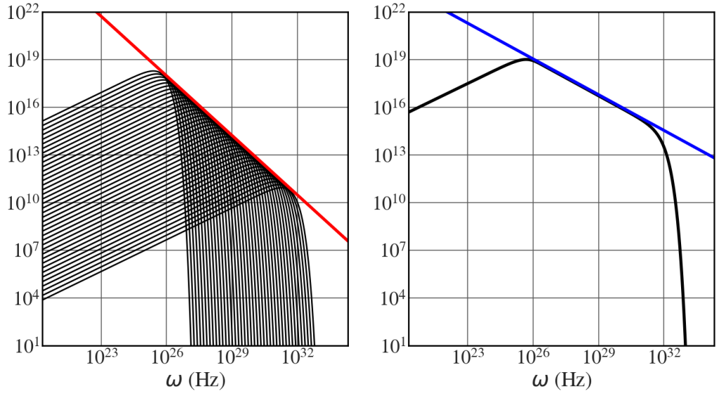
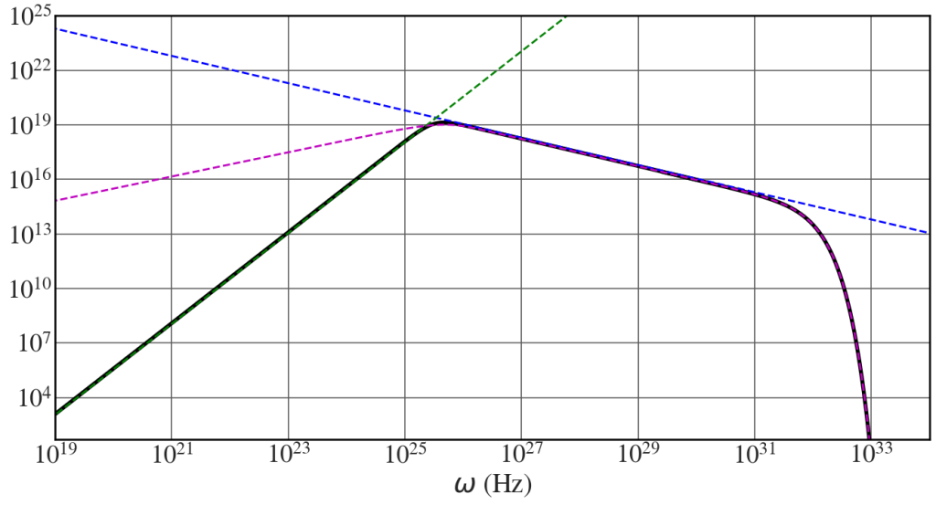
Qualitative spectral distribution of the synchrotron light emitted by an ensemble of charged particles
Qualitative synchrotron radiation spectrum, including self-absorption. See Fig. 9.12.
|
1 2 3 4 5 6 7 8 9 10 11 12 13 14 15 16 17 18 19 20 21 22 23 24 25 |
omega1 = np.logspace(14,30,50000) omega = np.logspace(14,36,50000) om2 = 1.0e32 kk = 0.2e-24 func1 = 1e60/(1e-23*omega1**3.252 + 1e60*omega1**(-0.002)) with plt.style.context(('seaborn-v0_8-whitegrid')): plt.rcParams.update(synchrotron_style) fig, ax= plt.subplots(figsize=(16,7.8)) ax.loglog(omega1, 3.5e-45*omega1**(2.5)*(func1) , lw=4, c='k') ax.loglog(omega[35000:], tot_power[35000:], lw=4, c='k') ax.loglog(omega, 3.5e38*omega**(-0.75), lw=2, c='b', ls='--') ax.loglog(omega, 3.5e-45*omega**(2.5), lw=2, c='g', ls='--') ax.loglog(omega, tot_power, lw=2, c='m', ls='--') ax.set_ylim(1e1,1e25) ax.set_xlim(1e19,1e34) ax.tick_params(axis='x', labelsize=26, pad = 5) ax.tick_params(axis='y', labelsize=26) ax.set_ylim(5e1,1e25) ax.set_xlabel('$\\omega$ (Hz)', fontsize=28, labelpad=3) plt.show() |
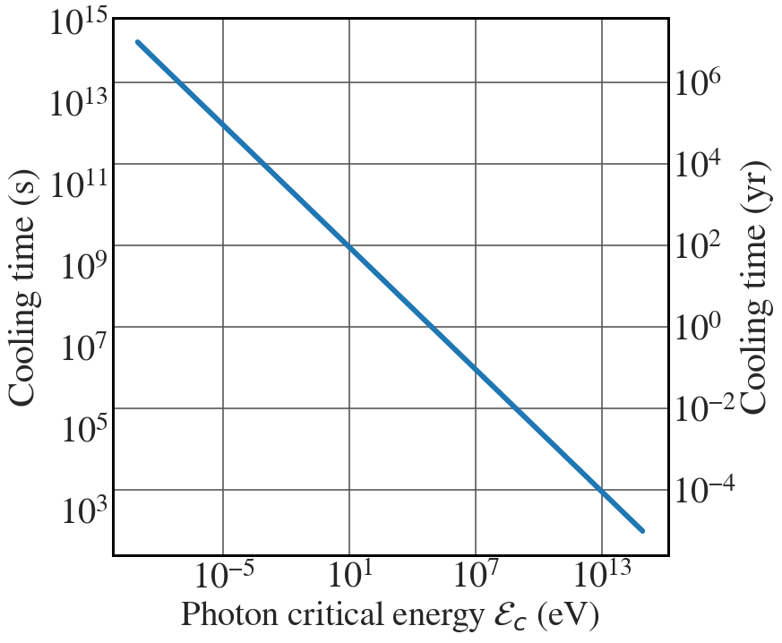
Synchrotron cooling time
See Fig. 9.14.
|
1 2 3 4 5 6 7 8 9 10 11 12 13 14 15 16 17 18 19 20 21 22 23 24 25 26 27 28 29 30 31 32 33 |
e = 1.602e-19 #C m = 9.10938356e-31 #kg c = 3.0e8 #m/s B = 5e-8 #T epsilon_0 = 8.854e-12 #F/m hbar = 6.5821e-16 # eV s gamma = np.logspace(1,13,2000) beta = np.sqrt(1.0-1.0/gamma**2) omega_c = 3*e*B*gamma**2 / (2*m) en_c = hbar*omega_c P_avg = (e**2 *B*gamma*beta)**2 / (9*np.pi*epsilon_0*m**2*c) tau_s = gamma*m*c**2 / P_avg tau_y = tau_s/31556909 with plt.style.context(('seaborn-v0_8-whitegrid')): plt.rcParams.update(synchrotron_style) fig, ax= plt.subplots(figsize=(8,7.8)) ax.loglog(en_c, tau_s, lw=4) ax.tick_params(axis='x', labelsize=29, pad=5) ax.tick_params(axis='y', labelsize=29) ax.set_xlabel('Photon critical energy $\\mathcal{E}_{c}$ (eV)', fontsize=28, labelpad=3) ax.set_ylabel('Cooling time (s)', fontsize=30, labelpad=3) ax2 = ax.twinx() ax2.loglog(en_c, tau_y, lw=4) ax2.tick_params(axis='y', labelsize=29) ax2.set_ylabel('Cooling time (yr)', fontsize=30, labelpad=3) ax.grid(False,axis='y') plt.show() |
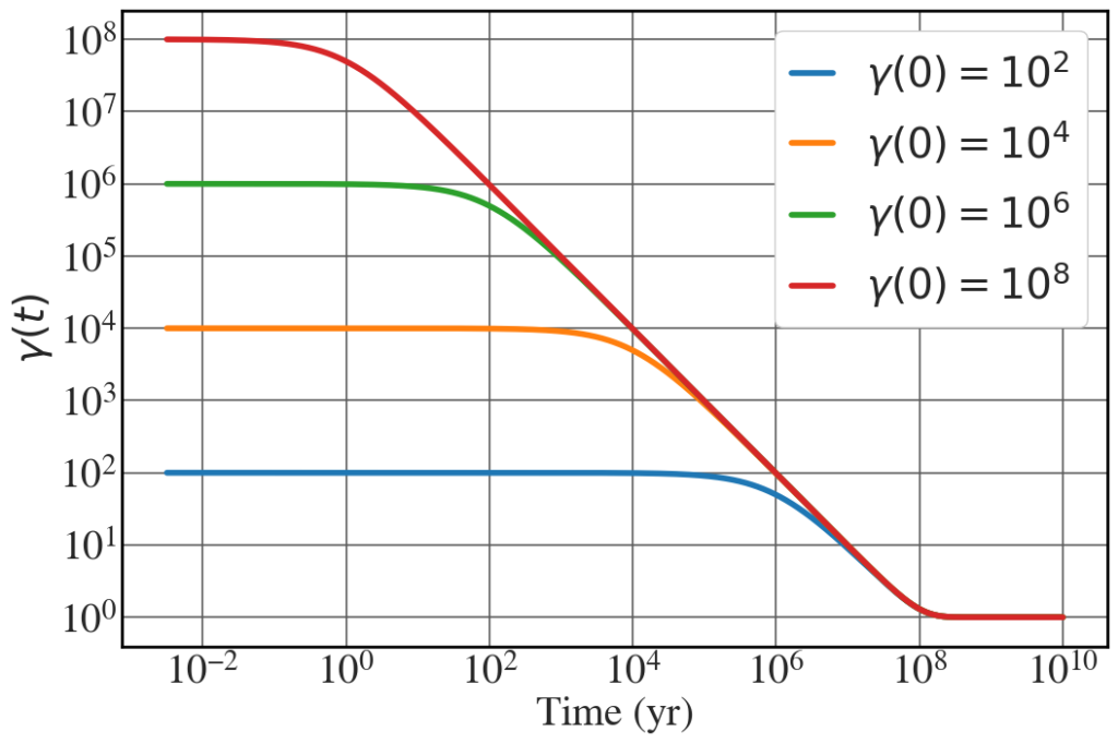
Synchrotron cooling: numerical calculation of the time-dependent Lorentz factor
See Fig. 9.15.
|
1 2 3 4 5 6 7 8 9 10 11 12 13 14 15 16 17 18 19 20 21 22 23 24 25 26 27 28 29 30 31 32 33 |
e = 1.602e-19 #C m = 9.10938356e-31 #kg c = 3.0e8 #m/s B = 5e-8 #T epsilon_0 = 8.854e-12 #F/m # Define the constant A = (e**2 *B)**2 / (9*np.pi*epsilon_0*m**3*c**3) t = np.logspace(5,17.5,100000) with plt.style.context(('seaborn-v0_8-whitegrid')): plt.rcParams.update(synchrotron_style) fig, ax= plt.subplots(figsize=(12,7.8)) gamma_label = ['$10^{2}$', '$10^{4}$', '$10^{6}$', '$10^{8}$'] for k, gamma_0 in enumerate([100,10000,1000000,100000000]): gamma = np.zeros_like(t) gamma[0] = gamma_0 for i,j in enumerate(t[:-1]): gamma[i+1] = gamma[i] - A*(gamma[i]**2 - 1)*(t[i+1]-t[i]) ax.loglog(t/31556909, gamma, lw=4, label='$\\gamma(0) =$'+gamma_label[k]) ax.tick_params(axis='x', labelsize=28, pad=5) ax.tick_params(axis='y', labelsize=28) ax.set_ylabel('$\\gamma(t)$', fontsize=28, labelpad=3) ax.set_xlabel('Time (yr)', fontsize=28, labelpad=3) plt.yticks(np.logspace(0, 8, 9)) plt.legend(fontsize = 28, frameon=True, framealpha = 1, handlelength = 1) plt.show() |
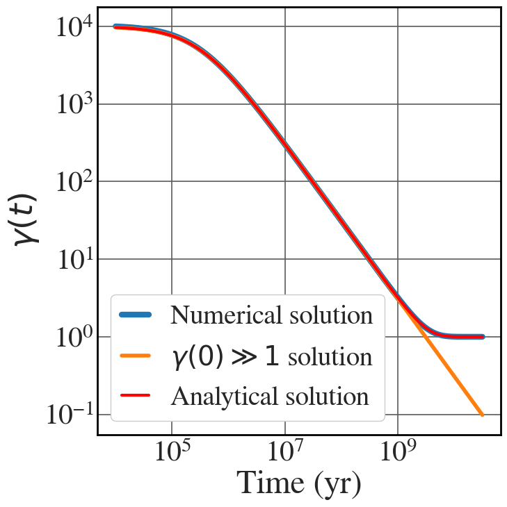
Synchrotron cooling: comparison of numerical and closed-form solution
See Fig. 9.16.
|
1 2 3 4 5 6 7 8 9 10 11 12 13 14 15 16 17 18 19 20 21 22 23 24 25 26 27 28 29 30 31 32 |
e = 1.602e-19 #C m = 9.10938356e-31 #kg c = 3.0e8 #m/s B = 5e-5 #T epsilon_0 = 8.854e-12 #F/m A = (e**2 *B)**2 / (9*np.pi*epsilon_0*m**3*c**3) t = np.logspace(4,10.5,500000) gamma = np.zeros_like(t) gamma[0] = 1e4 for i,j in enumerate(t[:-1]): gamma[i+1] = gamma[i] - A*(gamma[i]**2 - 1)*(t[i+1]-t[i]) A_cal = (gamma[0] - 1)/(gamma[0] + 1) with plt.style.context(('seaborn-v0_8-whitegrid')): plt.rcParams.update(synchrotron_style) fig, ax= plt.subplots(figsize=(8,8)) ax.loglog(t, gamma, lw=6, label="Numerical solution") ax.loglog(t,gamma[0]/(1+A*gamma[0]*t), lw=4, label="$\\gamma(0) \gg 1$ solution") ax.loglog(t, (1 + A_cal*np.exp(-2*A*t)) / (1 - A_cal*np.exp(-2*A*t)), 'r',lw=3, label="Analytical solution" ) ax.tick_params(axis='x', labelsize=30, pad=7) ax.tick_params(axis='y', labelsize=30) ax.set_ylabel('$\\gamma(t)$', fontsize=34, labelpad=3) ax.set_xlabel('Time (yr)', fontsize=34, labelpad=3) plt.legend(fontsize = 28, frameon=True, framealpha = 1, handlelength = 1) plt.tight_layout() plt.show() |
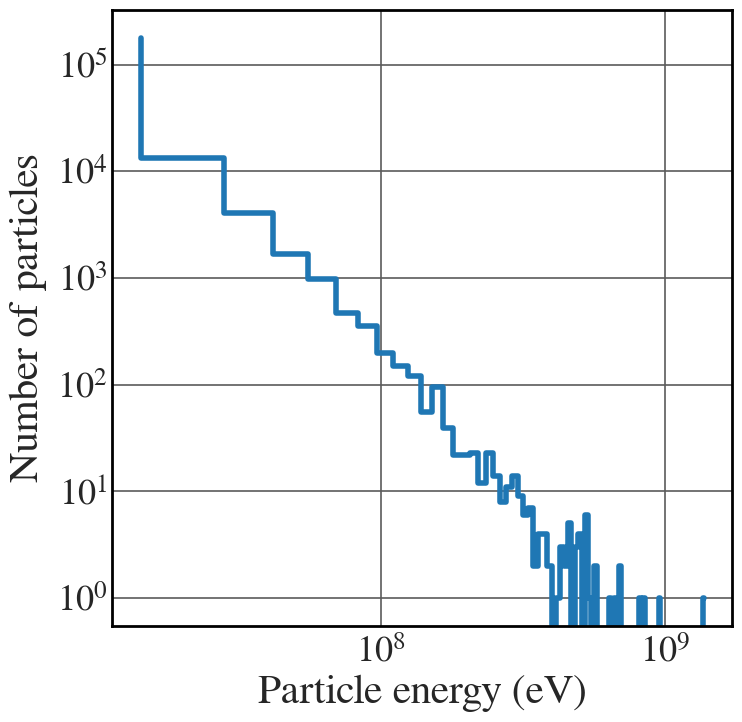
Fermi model for the acceleration of cosmic rays
See Fig. 9.21. Note: the code implements a Monte Carlo simulation, hence the plot will generally be different from the one reproduced in the figure, depending on the initialisation of the random number generator.
|
1 2 3 4 5 6 7 8 9 10 11 12 13 14 15 16 17 18 19 20 21 22 23 24 25 26 27 28 29 30 31 32 33 34 35 36 37 38 39 40 41 42 43 |
def fermi_acceleration(n_particles,n_epochs, V, gamma_init, p_esc): # Start with a monochromatic set of particles gamma_particles = gamma_init*np.ones(n_particles) for i in range(n_epochs): # Particles can escape the region with probability p_esc prob1 = np.random.rand(gamma_particles.shape[0]) mask1 = prob1 > p_esc gamma_particles=gamma_particles[mask1] # The particles that are not lost, can either be accelerated or decelerated prob2 = np.random.rand(gamma_particles.shape[0]) beta_particles = np.sqrt(1.0-1/gamma_particles) p_plus = (beta_particles + beta_mag)/(2*beta_particles) # particles that gain energy mask_plus = prob2 <= p_plus gamma_particles[mask_plus] = gamma_particles[mask_plus] + \ 2*gamma_particles[mask_plus]*beta_particles[mask_plus]*V/c # particles that lose energy mask_minus = prob2 > p_plus gamma_particles[mask_minus] = gamma_particles[mask_minus] - \ 2*gamma_particles[mask_minus]*beta_particles[mask_minus]*V/c return gamma_particles c = 3e8 beta_mag = 1e-2 V = beta_mag * c rest_energy = 0.511e6 with plt.style.context(('seaborn-v0_8-whitegrid')): plt.rcParams.update(synchrotron_style) fig, ax= plt.subplots(figsize=(8,8)) h, bins = np.histogram(rest_energy*gamma_final, bins=100) ax.loglog(bins[1:],h, drawstyle='steps', lw=4) ax.set_xlabel('Particle energy (eV)', rotation=0, fontsize=30) ax.set_ylabel('Number of particles', fontsize=30, labelpad = 7) ax.tick_params(axis='x', labelsize=26, pad=7) ax.tick_params(axis='y', labelsize=26) plt.show() gamma_final = fermi_acceleration(200000,5000, V=V, gamma_init=5, p_esc=1e-6) |
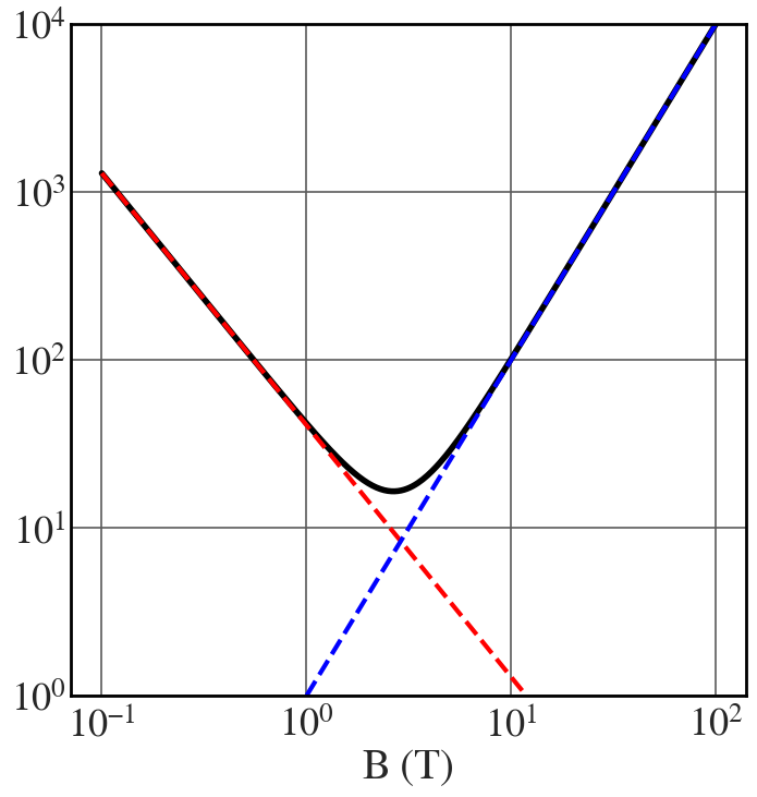
Energy equipartition
See Fig. 9.22.
|
1 2 3 4 5 6 7 8 9 10 11 12 13 14 15 16 |
eta = 40 # As measured in cosmic rays B = np.linspace(0.1,100,1000) U = (1+eta)*B**(-1.5) + B**2 with plt.style.context(('seaborn-v0_8-whitegrid')): plt.rcParams.update(synchrotron_style) fig, ax= plt.subplots(figsize=(8,8)) ax.loglog(B,U, 'k',lw=4) ax.loglog(B, (1+eta)*B**(-1.5), 'r--', lw=3) ax.loglog(B, B**2, 'b--', lw=3) ax.set_ylim(1,1e4) ax.tick_params(axis='x', labelsize=26, pad = 7) ax.tick_params(axis='y', labelsize=26) ax.set_xlabel('B (T)', fontsize=28, labelpad=3) plt.show() |
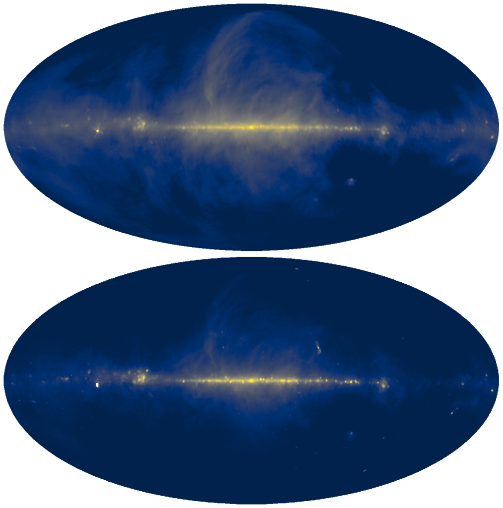
All-sky radio survey
The data plotted in the all-sky radio survey maps of Figs. 9.32 and 9.33 can be downloaded at the following pages:
The following code generates the maps in Fig. 9.32.
|
1 2 3 4 5 6 7 8 9 10 11 12 13 14 15 16 17 18 19 20 |
from astropy.io import fits haslam = "radio-data/haslam408_mollweide_dsds_Remazeilles2014.fits" sve = "radio-data/lambda_mollweide_STOCKERT+VILLA-ELISA_1420MHz_1_256.fits" data1 = np.flipud(fits.getdata(haslam)) data2 = np.flipud(fits.getdata(sve)) mask1 = data1 != 0 data1_ad = exposure.equalize_hist(data1, nbins=256, mask=mask1) mask2 = (data1_ad == data1_ad.min()) fig, axs = plt.subplots(2,1, figsize=(16,14)) data1_ad[mask2] = 0 p1 = axs[0].imshow(np.log(data1), cmap='cividis', vmin=3, vmax=6.8) axs[0].set_axis_off() p2 = axs[1].imshow(np.log(data2), cmap='cividis', vmin=8.2, vmax=10) axs[1].set_axis_off() plt.tight_layout() plt.show() |
The following code generates the close-up contour maps in Fig. 9.33.
|
1 2 3 4 5 6 7 8 9 10 11 12 13 14 15 16 17 18 19 20 |
with plt.style.context(('seaborn-v0_8-whitegrid')): plt.rcParams.update(synchrotron_style) fig, axs = plt.subplots(2,1, figsize=(10,12)) p1 = axs[0].contourf(np.log10(data1[768:-768,1536:2560]), cmap='cividis',levels=15)#, vmin=4) axs[0].contour(np.log10(data1[768:-768,1536:2560]), levels=15, colors='k') axs[0].set_axis_off() p2 = axs[1].contourf(np.log10(data2[384:-384,768:1280]), cmap='cividis',levels=15)#, vmin=8.4) axs[1].contour(np.log10(data2[384:-384,768:1280]), levels=15, colors='k')#, vmin=8.4) axs[1].set_axis_off() cb1 = fig.colorbar(p1, ax=axs[0]) cb2 = fig.colorbar(p2, ax=axs[1]) cb1.set_label('$\\log_{10}(T)$', size=30) cb1.ax.tick_params(labelsize=26) cb2.set_label('$\\log_{10}(T)$', size=30) cb2.ax.tick_params(labelsize=26) plt.tight_layout() plt.show() |
![]()
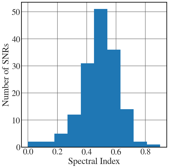
Spectral-index occurrences for shell-type supernova remnants
See Fig. 9.34. The data for these plots have been downloaded from A Catalogue of Galactic Supernova Remnants (Dave Green, Astrophysics Group, Cavendish Laboratory, Cambridge, UK). At the time of writing, we used the “2006 June” version of the catalogue. A newer version, “2024 October” has since been made available.
|
1 2 3 4 5 6 7 8 9 10 11 12 13 14 15 16 17 18 19 |
# csv file extracted from the web page https://www.mrao.cam.ac.uk/surveys/snrs/snrs.data.html snr_data = pd.read_csv("radio-data/snr_data.csv") # Select only the object with known spectral index, i.e. neglect the question marks and the "varies" mask_q = snr_data["spectral index"].str.endswith('?').values mask_v = snr_data["spectral index"].str.endswith('s').values mask = np.logical_and(np.logical_not(mask_q),np.logical_not(mask_v)) spectral_index = snr_data["spectral index"].values[mask].astype('float32') sup_type = snr_data["type"].values[mask] with plt.style.context(('seaborn-v0_8-whitegrid')): plt.rcParams.update(synchrotron_style) fig, ax= plt.subplots(figsize=(8,8)) ax.hist(spectral_index, bins=10) ax.set_xlabel('Spectral Index', rotation=0, fontsize=28) ax.set_ylabel('Number of SNRs', fontsize=28) ax.tick_params(axis='x', labelsize=26) ax.tick_params(axis='y', labelsize=26) plt.show() |
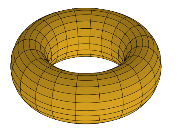
Torus
See Fig. 9.41. Example adapted from the Example E7.26 of C. Hill (2020) Learning Scientific Programming with Python (2nd edition), Cambridge University Press, Cambridge.
|
1 2 3 4 5 6 7 8 9 10 11 12 13 14 15 16 17 18 19 |
n = 100 theta = np.linspace(0, 2.*np.pi, n) phi = np.linspace(0, 2.*np.pi, n) theta, phi = np.meshgrid(theta, phi) c, a = 3, 1 x = (c + a*np.cos(theta)) * np.cos(phi) y = (c + a*np.cos(theta)) * np.sin(phi) z = a * np.sin(theta) fig = plt.figure(figsize=(15,15)) ax = fig.add_subplot(111, projection='3d') ax.set_zlim(-3,3) ax.plot_surface(x, y, z, rstride=5, cstride=5, color='goldenrod', edgecolors='k') ax.view_init(36, 26) ax.set_axis_off() plt.tight_layout() plt.show() |